Measuring Variations in Credit Risk among Markets: A New Product from Collateral Analytics

By James R. Follain and Michael Sklarz

Collateral Analytics has recently developed a new Credit Risk Model. It is designed to measure the losses due to borrower default on residential mortgages. The summary measure is the credit risk spread (CRS). It is defined as the sum of the annual expected losses due to default plus the cost of capital needed to insure against an extreme or stress scenario in house prices. A central theme of the model is to highlight variations in the CRS among metropolitan housing markets.

The purpose of this short article is to provide a case study using the new CA CR Model. The goal is to highlight variations in the CRS among markets and the types of mortgage products where such variations are likely to be most substantial. A key local market condition driving the variations is the set of future HP scenarios fed into the model, which vary by local market. The other critical driver of these variations is the inherent riskiness of the mortgage itself. Briefly, mortgages with relatively high initial LTVs and low credit scores will be the ones with the most variation among markets. Those with relatively low LTVs and high credit scores may also vary among markets but the variation will be much smaller because the average CRS for these loans is quite small. The intuition is this. Low LTV loans are much less sensitive to shocks in future house prices because the borrowers have substantial equity in the homes that will typically not be eliminated except in the worst of HP declines.

To demonstrate this aspect of the CRM a batch job was done for three different loans with widely varying credit risk. The low risk loan consisted of an initial LTV of 50 percent and a credit score of 800. The high risk loan had an initial LTV of .95 and a credit score of 660. An intermediate risk loan had 80/700 LTV/credit score combination. The loans evaluated were all prime 30 year FRMs.  The CRS is computed for each of these loan types for each of the 29 MSAs covered separately by the CRM.[1]

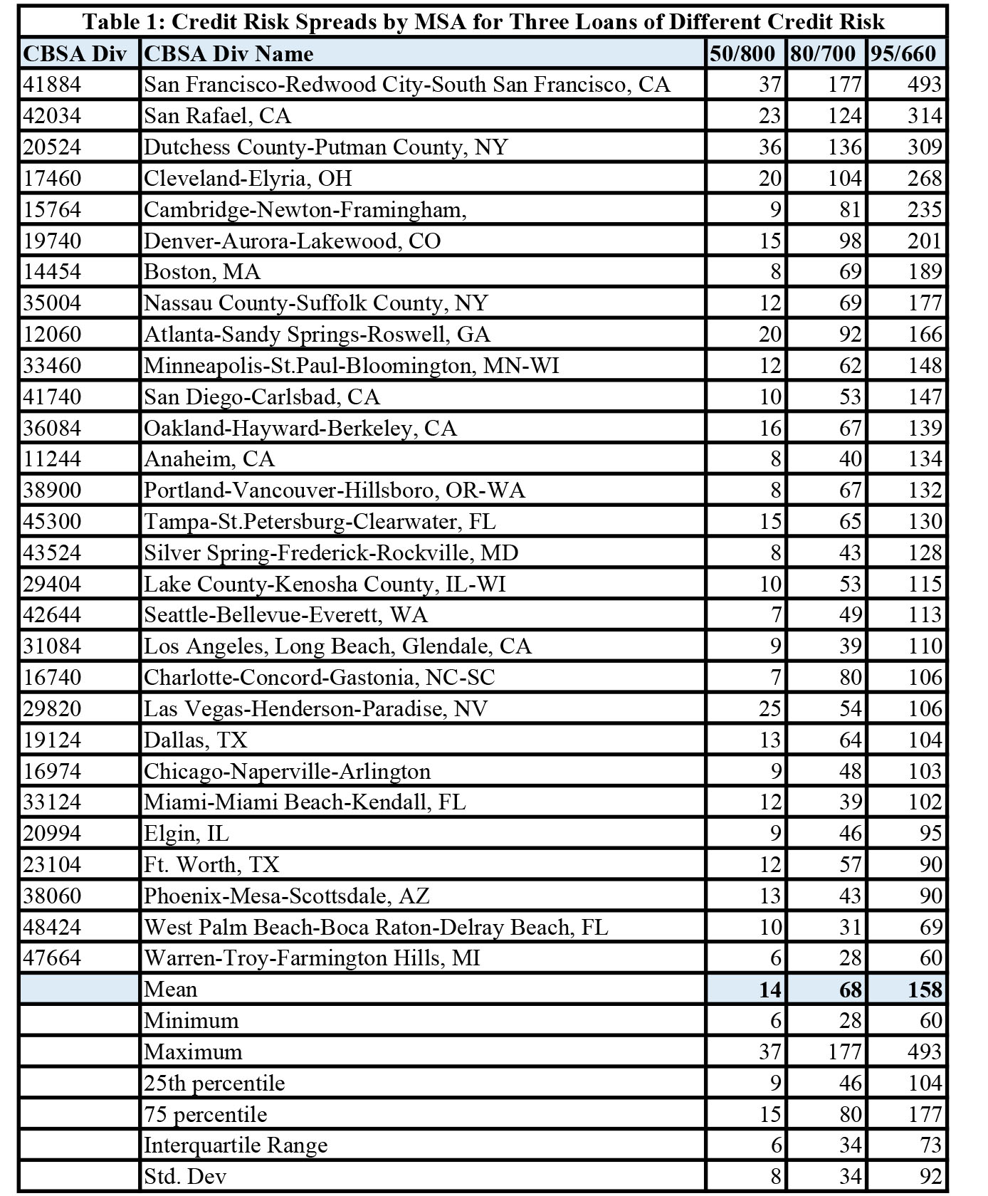
The main results of this batch job are captured in Table 1. Table 1 shows the CRS for three loan types and the results are ranked by the size of the CRS for the riskiest mortgage – 95 LTV/660 credit score. For this measure of credit risk, San Francisco has the highest amount at 493 bps and Warren, MI at 60. There is wide variation around the average of 158 bps. The interquartile range is 73 and the standard deviation among MSAs is 92 bps. Clearly, our measure of the CRS for this high risk loan varies widely among markets. The specific reasons for the variation are embedded in the complex calculations of the CRS, but the basic drivers include the different estimates of the default and prepayment equations, which affect the sensitivity of a shock to default from a house price decline, the specific house price scenarios fed through these equations, especially the stress scenario, and a variety of local traits such as the REO discount and recent employment growth.

At the other extreme is the distribution of the CRS for the least risky loan – the 50 LTV/800 credit score 30 YR FRM. These are highly correlated with the CRS on the risky loan – simple correlation of 77 percent; however, these are much smaller and much more tightly distributed that the CRS for the riskiest of the three loans evaluated. San Francisco also tops this list and Warren also has the lowest CRS for this loan. The mean CRS is only 14 bps and the standard deviation is 8 bps and the interquartile range is 6 bps.

The CR spreads for the third loan – 80 LTV/700 credit score – are between the other two, but they are sharply higher than the least risky loans. This is to be expected because as the LTV rises, the risk of default and the CRS rise more than proportionately. That is, an increase in the LTV by 10 percent from, say, 50 to 60 has a much smaller impact on the CRS than an increase in the LTV from 80 to 90 because the higher LTV loan is more sensitive to shocks in HP than the low LTV loan. The results for this intermediate risk loan are consistent with this idea, which is a well-established premise of the modeling of mortgage credit risk for many years. What is less established and what our model seeks to highlight is the variability in the CR spreads among markets even for loans with similar LTV and credit scores.

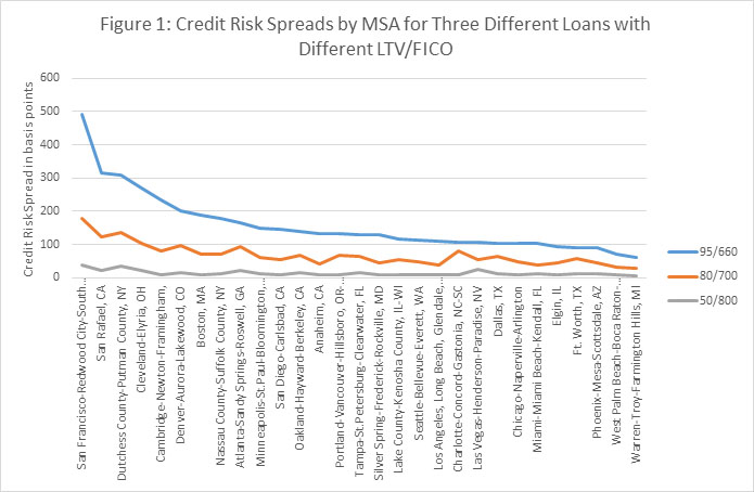
Figure 1 plots the three CR spreads by MSA. It captures the wide range of the CRS for the riskiest loan and the de minimum variation for the least risky loan.

One implication of this set of results is that the demand for the CA CR Model will be strongest for relatively risky loans. Here the lender or the investor in mortgages may benefit from the insights the model offers about variations in the CRS among markets. As this case study demonstrates, the variations among markets in the relatively risk loans can be substantial and pricing all mortgages of this risk class the same in all markets – one size fits all — may be a problem. On the other hand, the “one size fits all” may work just fine for mortgages with little credit risk like our 50 LTV/800 credit score example.

An obvious question is what drives the differences among MSAs for the same loan. This is a complex question because the number of components that define the CRS is substantial and difficult to disentangle. The drivers fall into three broad categories:

1.  The coefficients of the default and prepayment equations. There are
50+ coefficient estimates in each set of equations for each MSA.
The key ones pertain to the sensitivity of default to changes in the
current loan to value ratio over the life of the loan. MSAs in which the
sensitivity to increases to CLTV is largest will have higher credit risk
spreads, all else equal. These estimates reflect the historical experience
of default in these areas during the period 2003 until 2012.  Another
driver that varies among markets that enters the equations is the growth
rate in employment at the county level over the previous 12 months.

2.  The HP Scenarios fed into the equations. These include six scenarios
distributed around the mean or baseline forecast and one stress scenario.
Each of these consists of 5 years of projections of monthly forecasts.
These are generated by CA’s HP Model. So, one MSA may have higher
CR Spreads if the baseline is smaller, the stress scenario is more severe,
and the of the various HP scenarios around the baseline is more
dispersed. The third set consists of various factors that have their largest
impact on the Loss Given Default. These include the REO discount and
the average days to foreclosure in the state in which the MSA is located.

3.  A review of the results for this case study proves to highlight the
complexity of the interactions among these various drivers. For example,
the cumulative five year baseline (11 percent) and stress scenarios
(-17 percent) and the days to foreclosure (330) for San Francisco, the
MSA with the largest CRS, are rather modest in comparisons to these
values for this set of MSAs. However, examination of the coefficient
estimates in the default equation indicates that the predicted probability
of default is more sensitive to a decline in house prices than is the case
for the other MSAs. This is in contrast to the case for Dutchess County,
NY, the MSA with the third highest CRS in this case study. The baseline
HP scenario calls for much smaller growth (.04) and a more severe
stress scenario (-.17). The REO discount (.5) and the days to
foreclosure (820) are also much higher for Dutchess County and
work to increase its CRS.

The White Paper for the CRM contains more analysis of the drivers of the CRS among markets. Future articles and case studies will also seek to identify the most prevalent explanation for the variations. Until then, the results of this case study demonstrate that the variations in the CRS among markets will be highest for the riskiest loans. Also, those MSAs in which the sensitivity of the probability of default to shocks in house prices is greatest and those with the more pessimistic HP scenarios, REO discounts, and days to foreclosure will have the highest CRS.