by Dr. James R. Follain and Dr. Michael Sklarz
Overview
Collateral Analytics offers two types of Credit Risk Models (CRM). One focuses upon newly originated loans and generates various estimates of the credit risk associated with the future performance of the model. Key indicators include the annualized credit risk spread (CRS), the amount of capital needed to protect against stress scenario credit losses (capital), and an estimate of the present value of future cash flows net of future default losses (MortvaltoUPB). These indicators are computed for five years into the future and for seven different house price scenarios. An important theme of the results is the wide variation in these indicators among local housing markets.
The second and newest CR Model is the subject of this short article. The seasoned CRM focuses upon the evaluation of credit risk in performing mortgages loans. Seasoned loans are ones that have been originated at some point in the past. Some of these traits are fixed at origination such as the initial mortgage rate for fixed rate mortgage and some vary over the life of the loan such as the amount of the outstanding UPB, the gap between the initial mortgage rate, and the current loan to value ratio. For example, a seasoned loan may be a FRM with a 30 year maturity originated in 2007. The goal of the seasoned loan model is to provide information about the credit risk associated with the mortgage. The results of the seasoned model are provided as of today’s date and, like the CRM for new loans, and at the end of a five year forecast beyond today’s date.
There are a number potential applications for the model. One is for portfolio lenders to seek additional information about the credit risk in its portfolio and the capital required to meet stress scenarios. Another is for potential investors to assess the potential value and risk associated with the loan. It may also raise potential flags about internal models that, perhaps, fail to pick up elements of risk not typically covered by standard credit risk models.
This report discusses the results of a case study of 263 seasoned loans originated between 2003 and 2007 in four California MSAs: Anaheim; Los Angeles; San Diego; and San Francisco. After a review of the initial traits of these loans, the discussion of the results focuses upon key indicators at the current age of the loan and those based upon a five year projection of loan performance under varying HP scenarios. A theme to the results is that these loans appear to be strong candidates for refinancing since they have relatively low current LTVs and substantial gaps between the initial contract rate and the current 30 year FRM rate of 4.16 percent. Alternatively, these loans seem to be good candidates for 2nd lien home equity loans, since these second loans would rest upon strongly performing first loans with relatively low LTVs.
Key Inputs to the Case Study
The seasoned loan model has the capacity to evaluate a wide set of loan traits. The particular sample chosen for this study consists of 263 prime 30 year FRM loans from the Lewtan data set that were still active as of August 2014. These were chosen from the four large MSAs in California: Anaheim; Los Angeles; San Diego; and San Francisco. About 82 percent were 30 year maturities and the other 18 percent had 15 year maturities. Several other key traits of these loans are captured in Table 1.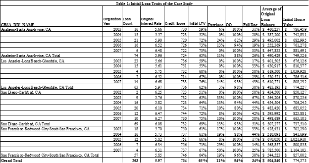
The main point to be taken from this table is that these loans were generally of high quality with relatively modest credit risk at the time of origination. The best indicator of this is that the average loan to value ratios at origination were quite modest. Only one exceeded 80 percent and the overall average initial LTV is 65 percent. Likewise, the credit scores are quite high. The overall average credit score is 734. Only 7 were below 660 and none were below 620. Most were made for the purpose of refinancing (89 percent) and only 11 percent were made to purchase the property. 94 percent of the borrowers were the owner occupants. These are all consistent with the notion of a prime loan. Nonetheless, 34 percent had fully documented mortgage applications and 66 percent had something less than full documentation. Most were for the purpose of refinancing (89 percent) versus only 11 percent for the purpose of home purchase.
The average initial loan balance was $500,000, which is above the conforming loan limits for loans eligible for purpose by the GSEs during these years. For example, about 75 percent of these loans are above the conforming loan limit of $417,000 in 2007. As a result, these are largely loans purchased for non-agency MBS. The average value of the property for these loans was about $775,000.
Another key aspect of the input information is the level of the initial interest rate. The overall average is about 6 percent (5.97) and the variation of these rates among origination year is quite consistent with the market rates of those years. For example, the average 30 year FRM increased from 5.84 to 6.34 from 2003 to 2007, which is quite consistent with the data in Table 1.
Results as of August 2014
A number of results are computed for these loans as of August 2014. Some are based upon straightforward calculations based upon the initial loan traits and some are based upon the default and prepayment equations underlying the seasoned loan model. These are summarized in Table 2.
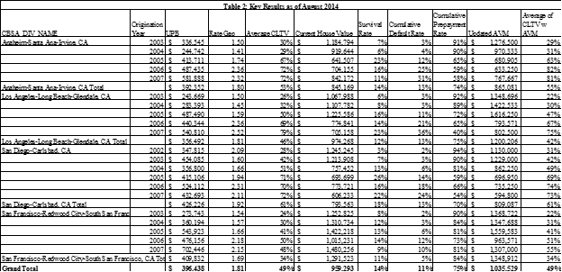
The average UPB is now about 20 percent lower than the average initial balances, which is based upon normal amortization rates of 30 and 15 year FRMs. One key point to note about these results is that these loans all have initial contract rates well above the 30 year FRM market rate of interest in August 2014, which was 4.16 percent. The average gap between the initial contract rate and the current mortgage rate as of August 2014 is about 180 basis points. A common rule of thumb in years past is that a borrower would typically refinance if such a gap neared or exceeded 200 bps if the current LTV was 80 percent or less. In fact, these criteria are met for most of these loans. The average LTV as of August 2014 is about 50 percent, down from 65 percent based upon increased values of the properties from an average of $775,000 to about $980,000. Indeed, the seasoned credit risk model predicts very high prepayment rates for these loans as of August 2014. The average predicted cumulative prepayment rate is about 75 percent.
The cumulative predicted default rate is about 11 percent, which is likely due to the volatility of house prices during the early years of these mortgages when the model would have predicted relatively high monthly default rates. The overall average predicted survival rate for these loans is only 14 percent. In brief, these loans seem more than ripe for refinancing according to common rules of thumb and the predictions of our prepayment and default equations. Alternatively, these loans seem very appropriate for the addition of 2nd lien home equity loans because they would be on top of very strongly performing first liens.
This case job also provides an opportunity to provide numerous comparisons of the value of the initial appraisals underlying the loan and changes in these values using various CA valuation information. Table 3 offers information on various comparisons that can be made.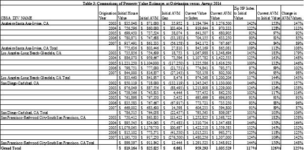
First, note the two different ways of measuring value at origination – initial house value used for the loan (column 3) and CA’s retrospective AVM for the property on the origination date (column 4). The average AVM value is $825,825 and the average initial appraised value is $819,825. The AVMgap (column 5) is $6,661, which is less than one percent of the average assessed value. That is, the two series are highly correlated. Having said this, there is wide variation around this average gap. Indeed, our default equation includes a variable that measures the AVM gap adjusted for confidence score. A key result is this: the larger the negative AVM gap (AVM less than the initial appraised value), the larger the probability of default and the higher the credit risk spread on a loan, all else equal. The role of this variable is discussed in more detail in a recent CA article: Measuring the Impact of Upwardly Biased Appraisals on Credit Risk. The predicted default rates discussed above incorporate these initial AVM gaps.
Second, the results provide two approaches to compare the changes in the values of these properties house prices from origination until August 2014. Understanding the changes in the values of these properties over the life of the mortgage is critical to the measurement of the credit risk embodied in the loan because the critical driver of default in mortgages is the updated or current loan to value ratio. Many previous analyses of this ratio rely upon national, state, and, sometimes, local market indexes of house prices. One of the two CA approaches in the seasoned model updates the values using CA ZIP Code indexes of the price per square foot of properties (column 5). The CA Credit Risk models uses these local market indexes to update the current loan to value ratio. The seasoned loan model offers a second approach — an updated AVM as of August 2014 (column 6).
A comparison of these values for August 2014 shows that the AVM values generally show greater appreciation than the ZIP Code level indexes. The average AVM value in August 2014 is $1,035,529 versus the indexed based value of $959,293. There is variation around this pattern. In particular, the AVM values show much less appreciation in the AVM than the local indexes for Anaheim in 2006/7, LA in 2002, and SF in 2007. The output of the seasoned loan model offers the opportunity to dig more deeply into these differences.
Projected Performance for Five Years
The final set of results from the seasoned loan credit risk model pertain to five year projections of the future cash flows from the mortgage. These are based upon seven different house price scenarios, one of which is the severe stress scenario. These scenarios vary among local housing markets at the MSA level. Several summary measures are focused upon in this report. The first three are extensions of the three summary measures offered as of August 2014 – the predicted cumulative survival, default, and prepayment rates. The other two are the amount of capital required to protect against a severe downturn in house prices (capital) and an estimate of the future value of the cash flows from the mortgage (Mortgage Value). These results are summarized in Table 4.
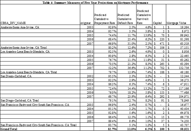
The first three tell the same basic story told by the results as of August 2014. That is, these mortgages are strong candidates for refinance or early prepayment. The average cumulative prepayment rate is 83 percent versus 75 percent as of August 2014. The predicted default rate is also relatively low at 11 percent, which is about the same as of August 2014. The predicted survival rate is now just 6 percent. Again, the model strongly predicts that these loans are strong candidates for early prepayment and the risk of default is small.
The two other summary measures also paint a similar story both of which stem from the very small predicted survival rates. Capital averages a mere $100 because the likelihood of the loan surviving is near zero owing to the high expected prepayment rates. The other measure is also driven by the low survival rate. It equals the present value of future mortgage payments plus the future value of early prepayments and less future losses due to default. These are all weighted by the survival rate hence the sum of these numbers if quite small.
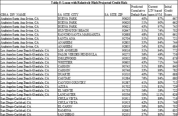
Of course, there are exceptions to this rather pristine picture of these loans. Twenty five loans have predicted default rates of at least 30 percent. Information about them is provided in Table 5. These tend to have either relatively high current LTVs as of August 2014 and relatively low initial credit scores. They are distributed widely among the four MSAs. These would be loans worthy of a much closer look by potential investors and other CA AVM products.
An obvious question is why these loans are still “alive” and payments are being made on a regular basis with little evidence of delinquencies. Several possible explanations come to mind. They deal with the generic problem that the information available to the model is omitting potentially valuable and updated information. For example, perhaps the incomes of the borrowers and their credit scores have declined since origination, which would make refinancing in today’s relatively stringent refinancing market difficult. Also, perhaps there are second liens on top of the first that may hinder refinance. The client may wish to search for this additional information to help understand why the loans are still current. Also, perhaps the properties have changed and their values are lower than CA’s AVM can capture. Application of more thorough AVM processes and evaluation of more information about these specific properties might reveal an explanation as to why the mortgage have not prepaid. Of course, some of these borrowers may be relatively well off and content to simply pay off the loans as scheduled. However, the model strongly suggests, conditional on the information utilized, that these loans are strong candidates for refinancing in the near future.
Key Conclusions and Possible Extensions
A case study of 263 still performing loans has been conducted with CA’s seasoned credit risk model. The main conclusion is that the majority of these loans are strong candidates for early prepayment because they have relatively low current LTVs, relatively high initial credit scores, and, most importantly, have substantial gaps between their current mortgage rate and the current market rates for 15 and 30 year FRMs. As noted above, this conclusion suggests that more information about these loans could be obtained to help resolve the “puzzle”. These would include updated information about the credit scores and incomes of the borrowers and whether they have second liens. Some of this information could be readily obtained if the borrower applies for a 2nd lien home equity loan. Indeed, absent any negative trends in borrower income and credit scores and as noted above, these seem like strong candidates for home equity loans. Indeed, further investigation may reveal that many of them have already obtained home equity loans on top of their strongly performing first loans.
An opportunity to evaluate other portfolios of seasoned loans submitted by potential clients would provide further study on the CA CRM for Seasoned Loans. The same information offered in this case study and, perhaps, some of the other information noted above, can be provided in order to help clients evaluate the riskiness of these loans. The information may help develop capital assignments for these loans. In this particular case, lenders would be justified in providing much lower capital amounts than would typically be assigned for UPBs unadjusted for predicted risk. Also, potential investors may wish to use the information to help establish bid prices for the loans. On the one hand, the results suggest that there is little credit risk; on the other hand, investors should probably view this as a very short term investment since the likelihood of prepayment is so high. The information may lead investors to collect more information about these loans. Lastly, information from the seasoned CRM might be helpful in identifying borrowers who may be strong candidates for home equity loans.
Download a PDF file of this research paper here.