How CA’s Credit Risk Model Can Help
by Dr. James R. Follain and Dr. Michael Sklarz | Mar. 23, 2015
One of the important lessons of the recent house price bubble and bust cycle is the wide variation in the size of the boom and bust among housing markets and the associated fallout of the cycle. Follain and Sklarz (2014) use data at the ZIP Code level to demonstrate the enormous variability of house prices between 2005 and 2014 at the ZIP Code level.[i] The recently updated HP model underlying the CA Credit Risk Model also produces substantial evidence to demonstrate the key point – local market conditions play a critical role in the movement of house prices.[ii] Failure to incorporate such risk into the lending and investment decisions of banks and investors can lead to substantial concentrations of risk in those regions where the outlook for house prices is less optimistic. For example, failure to slow down the bubble in places like Stockton CA and other parts of the SAND states prior to the bust contributed to much more severe and negative outcomes in these areas.
Potential Remedies for Regional Concentrations of Credit Risk among Markets
A report by the OCC (2011) provides some background and motivation for lenders to address regional concentrations of credit risk.[iii] Here is one quote from the report: “Supervisors have long recognized that a large credit risk exposure to a single borrower or family of borrowers, when measured as a percentage of bank capital, poses a potential threat to a lending institution’s safety and soundness, and regulation has imposed a limit on such exposures for that reason. Because of that limitation, individual transactions rarely cause material losses or bank failures. Rather, pools of individual transactions that may perform similarly because of a common characteristic or common sensitivity to economic, financial, or business developments have been the primary cause of credit related distress. If the common characteristic becomes a common source of weakness, loans in the pool could pose considerable risk to earnings and capital.” The continued growth in mortgage landing in the SAND states (AZ, CA, FL, and NV) as the house price bubble grew and grew strikes us an example of what the OCC has in mind.
The OCC also offers advice on how to mitigate and combat such regional concentrations of risk. These include (see pp.12-13 of the OCC Report):
• Modifying underwriting standards in the affected regions, which can include increasing mortgage rates and tightening underwriting criteria in the affected regions
• Buying additional insurance or guarantees for loans in the affected region; and,
• Holding capital to compensate for the additional risks in the affected regions.
In hindsight, all of these could have been helpful in stemming the ultimate fallout of the last crisis had lenders had access to an appropriate tool kit to combat regional concentrations of mortgage credit risk and the commitment to employ it.
How CA’s Credit Risk Model Can Help
CA has developed its Credit Risk Model to help address the challenges of regional concentrations of mortgage credit risk. It does so by offering a variety of measures of such risk at the level of the metropolitan area. The core measure is what we call the credit risk spread, which is an annualized measure of the losses to a lender or investor due to mortgage default. Another measure is the prudent amount of economic capital needed to cover credit losses from residential lending in extreme or stress scenarios.
These measures are calculated using state of the art models of mortgage prepayment and default and, the critical ingredient, a variety of future house price scenarios for many metropolitan areas. In essence, the local house price scenarios and other local market information are fed through the default and prepayment equations to construct estimates of the Credit Risk Spread (CRS) and the capital associated with these scenarios, loan types, and locations. These two output measures are related but they are not identical. The full definition of the CRS = EL + (r – rf)*Capital, where EL is the annualized amount of expected credit losses, r is the normal rate of return on investments by the lender, rf is the risk-free rate of return, and capital equals the losses in the extreme stress scenario less expected losses over the first five years of the life of the loan. As such, capital is one component of the CRS that highlights losses during stress scenarios whereas the full CRS seeks to incorporate both expected and stress losses.[iv]
We highlight the results for two loan types. One is a relatively high credit risk loan with an initial credit score of 660 and an initial LTV of 90 percent –loan type 1. The other is less risky and has a credit score of 700 and an initial LTV of 80 percent – loan type 2. Otherwise, the traits of these two loans are those of a prime 30 year FRM. The values of the CRS 1 and 2 and CAPUPB1 and CAPUPB2 are contained in Table 1 for a subset of the 80 relatively large metropolitan areas evaluated for this case study. They are further distinguished in the table by those with relatively high and relatively low credit risk. High risk is defined as an area with values of the four measures that are above the 90 percentile values for the sample and low risk is defined as those below the 10 percentile values for the sample for 2 or more of the variables.
The ten with the largest amounts of credit risk have capital ratios for the riskier of the two loans near or above 5 percent and well above the average capital ratio for the 80 metro areas of 3 percent. The capital ratios for the less risky loan type are also well above the average ratio of 1 percent. Similarly, the two credit risk spreads for these 10 metropolitan areas are well above the average values of CRS 1 (85 bps) and CRS 2 (41 bps). These metro areas include regions around the country.
The ten with the smallest amounts of credit risk according to our weighting scheme include 9 with capital ratios for the riskier of the two loans near or below 1.3 percent, which is the 10th percentile value for the full sample. Los Angeles is an exception on this as the capital ratio for the riskiest loan is 2.3 percent. Los Angeles makes our list because it has relatively low values for CRS 1 (35 bps) and CRS 2 (19 bps). This group also includes areas from all over the country.
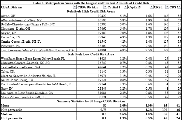
One possible strategy for a lender suggested by these results is to raise the rates it charges in the high risk areas and lower them in the low risk areas. This strategy faces a variety of obstacles in the mortgage industry as witnessed by the strong similarity of mortgage interest rates among metropolitan markets. As an example of such similarity, consider the most recent mortgage interest rate data reported by Freddie Mac in its survey of mortgage lending. The average rate on a 30 year FRM was 3.75 percent for the entire country. The highest rate among regions was 3.84 in the Southeast region and 3.70 in the Western Region. Though these are averages that may mask more variation within these regions, we are comfortable with our claim that mortgage rates at the area of the metropolitan level generally show much less variation than is suggested by our Credit Risk Model.
An alternative strategy is to keep rates the same as the local competition in a market but allow internal capital allocations to vary. In this case, capital would be increased in the high risk areas and lowered in the low risk areas. For example, capital on the prime 30 year FRM with an 80 LTV and a 700 credit score could be raised to 1.6 percent in Akron, OH and 2.5 percent in the San Francisco metropolitan area. This is well above the overall average capital ratio for this loan among the 80 metro areas in this study, which is 1 percent. The lender may also choose to lower its capital ratios in the relatively low risk areas. For example, the capital ratio on this standard prime loan could be between .5 and .8 percent among the low risk areas. With this strategy the lender is adjusting its internal economic capital to address regional concentrations in its risk while leaving its mortgage rate unchanged and similar to its competition in those areas.
Drivers of the Variations in Credit Risk among Markets
One obvious question is why do the measures of credit risk vary among these markets? In fact, the model is based upon a variety of factors that vary among the metropolitan areas. These include some metro specific prepayment and default equations, metro specific house price scenarios, loss given default (LGD) estimates, and the lagged growth rate in county employment, which is included in our default and prepayment models.
One challenge is identifying the impact of metropolitan area specific default and prepayment equations on the credit risk spreads. In anticipation of this we generated an alternative measure of credit risk that uses the same default and prepayment equations for all markets and metro area specific house price scenarios and all of the other assumptions used to estimate credit risk spreads. This measure is called CRS 3 and it, like CRS 1, pertains the credit risk on the loan in question, which is the loan with the 660 credit score and the 90 percent LTV. The difference between these two measures can serve as an indicator of the role of the metro area default and prepayment equations since they rely upon all of the same information except the default and prepayment equations. Consider the example of San Francisco. CRS 1 is 192 bps for this loan but CRS 3 is only 76. The only difference in the calculation is that separate default and prepayment equations are used for San Francisco to capture the behavior of borrowers in that area for CRS 1 whereas CRS 3 is based upon estimates of a default and prepayment equations using pooled data from many metro areas, including San Francisco. As such, the gap between the two – 192 less 76 – reflects the differences in the prepayment and default equations.
To shed light on the roles played by the various factors that drive CRS 1, consider a simple regression model that explains CRS 1 as a function of these key variables. Table 2 contains the results of the regression for the 80 metro areas.
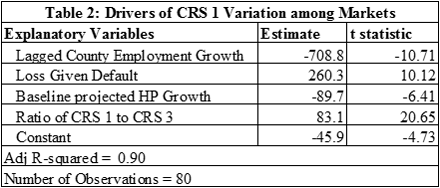
All of the drivers have the expected signs in both regressions.
• Counties in which lagged one year employment has been stronger have lower credit risk spreads;
• Large values of LGD (loss given default) increase credit spreads. LGD is a function of days to foreclosure and the REO discount, which are also market dependent.
• A larger projection of future house price growth for the baseline scenario reduces the credit risk spread for an area.
• Those areas with a larger ratio of CRS 1 to CRS 3 have larger credit spreads, which as discussed above, reflects the heightened sensitivity of default and prepayment using the metro specific default and prepayment equations relative to the pooled estimates of these equations.
These variables explain 90 percent of the variation in the credit risk spreads and all of the coefficient estimates are statistically significant.
Brief Summary
Lenders are encouraged by prudent internal financial management and regulators to be aware of variations in credit risk among regions. If the portfolio contains loans in areas thought to be of high credit risk, then prudent steps can involve raising rates or internal capital in the high risk areas. The CA Credit Risk Model provides an indicator of variations in credit risk among markets and two specific outputs to combat regional concentration of credit risk. One is to raise rates as suggested by the Credit Risk Spreads. Another is to leave rates the same but raise internal economic capital for loans from relatively risk regions of the country. This study offered very specific examples of how this might be done using CA’s Credit Risk Model.
Download a PDF file of this research paper here.
[i] Follain and Sklarz (2014) discuss this in a recent article in Housing Wire entitled: Here is strong proof of wide differences in local house prices.
[ii]Follain and Sklarz discuss CA’s latest House Price Model in a recent article on the CA web page: Description of the CA House Price Model and Key Assumptions Underlying the Model.
[iii] “Concentrations of Risk”, September 2011, OCC.
[iv] The CA Web site contains several articles about the Credit Risk Model; for example, see the April 2014 article by Follain and Sklarz Measuring Variations in Credit Risk among Markets: A New Product from Collateral Analytics.