by Michael Sklarz, Ph.D., Jim Follain Ph.D., and Norm Miller Ph.D.
Our most recent analysis of house prices provided insights about the potential threat of a house price bubble in various parts of the country. The primary indicator of a bubble is deemed to be the gap between the level of prices at a point in time and the predicted level of prices based upon a set of economic variables. The larger the gap or residual, the higher are actual prices relative to what the economic fundamentals suggest is appropriate for a particular market and time period. A variety of charts demonstrate the intuition underlying this analysis.
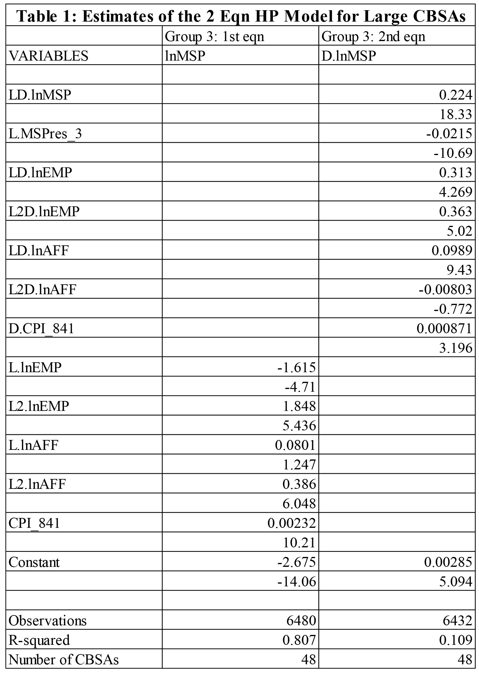
The purpose of this article is to take this argument one step further. A two equation model is estimated to produce forecasts of house prices for 48 large CBSAs over the next five years. The key distinguishing feature of the model is the incorporation of the residual as one of the explanatory variables. The first equation is similar to the one underlying the previous article: the level of prices in a particular quarter and CBSA is regressed against lagged values of the level of employment and the affordable price, and a national index of inflation. A second equation estimates the change in the level of prices as a function of the lagged growth rates in house prices, the two lagged values of the change in employment and the affordable price, the change in the national index of inflation, and, most importantly, the lagged value of the residual generated by the first equation.[i] All else equal, we expect future growth in the price of housing to be negatively related to the lagged value of the gap. [ii] The estimates of the two equation model are obtained by pooling data for 48 large CBSAs for the period 1981:q1 through 2015:q1. The estimates of the model are contained in Table 1 below. The first columns contains the estimates of the first equation and the second column contains the estimates of the second equation.
Important Model Results
The results confirm the powerful role that the lagged residual plays in the growth rate of house prices. The coefficient estimate is -.0215 and its t statistic is highly significant. For example, a 10 percent gap can lead to a reduction in prices of .215 percent in the following quarter, all else equal. Note, as well, that a higher lagged growth rate in house prices leads to faster growth in house prices and is consistent with the momentum affect often associated with bubble formation. The other coefficient estimates are consistent with expectations. In particular, higher levels of employment and employment growth and a higher affordable price and a growth in the affordable price increase the median sales price and its growth rate, all else equal.
Summary of the Five Year Forecasts
This two equation model is used to make five year projections of quarterly house prices for each of the 48 CBSAs. This requires a number of assumptions about the future values of the variables that drive the model. Our assumptions are these:
• The 30 year FRM, which affects the affordable price, increases from 4 percent in 2015 to 5 percent at 25 bps per year.
• Inflation is set equal to 4 percent per year.
• A vector autogression model (VAR) is used to project future values of the level of employment and household income, which is another factor that drives the affordable price. These VAR estimates are estimated separately for each CBSA and are intended offer future predictions that reflect long-term trends and relationships in these two variables.
• The residual gap declines by 5 percent per year during the forecast period beginning with its value in 2015:q1.
All of these assumptions can be adjusted in order to highlight the sensitivity of the predictions to these various assumptions.
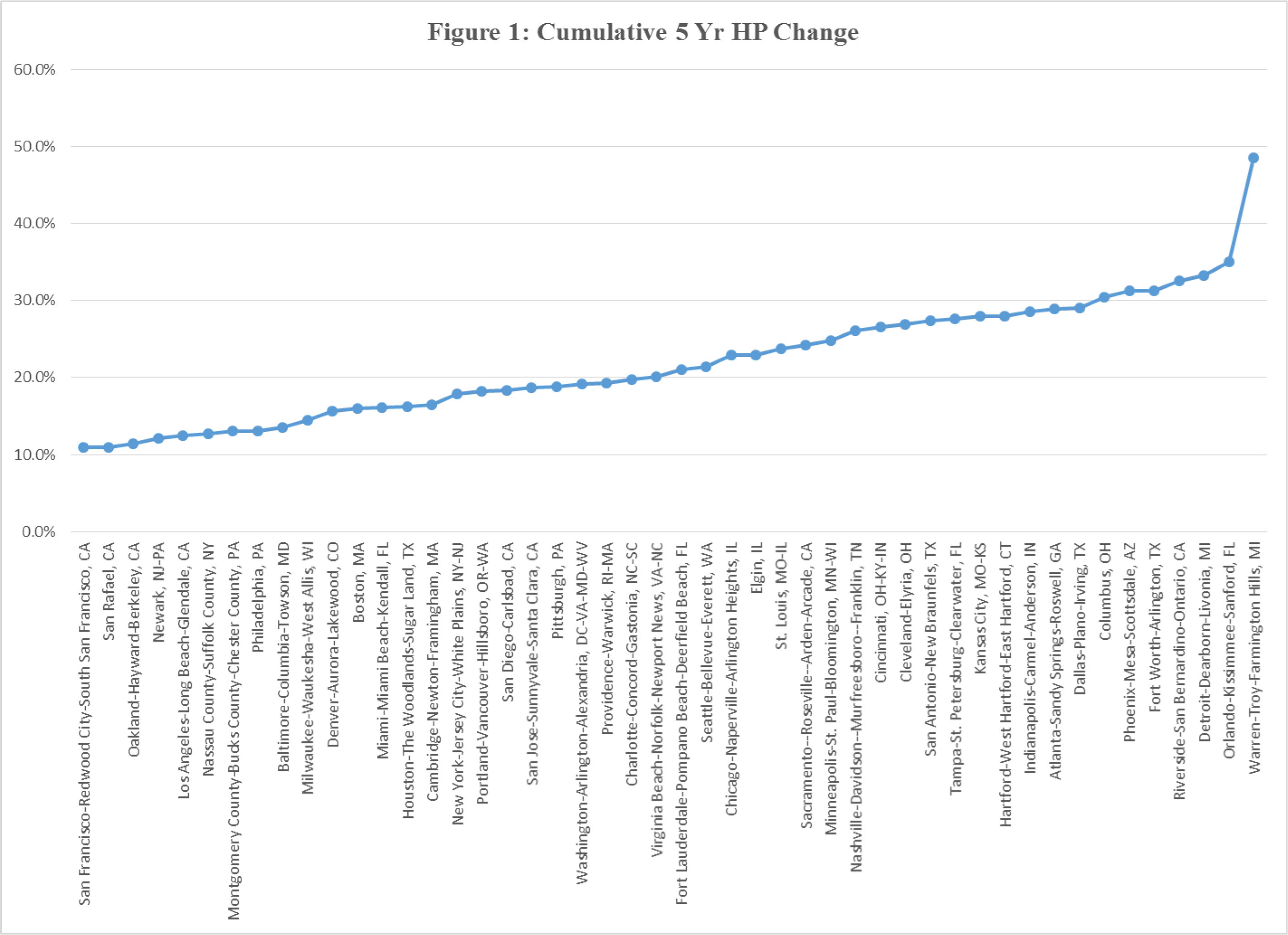
Two exhibits are used to present predictions of house prices for these CBSAs through the end of 2019. The first is Figure 1 above, which plots the cumulative predicted change in house prices by CBSA. These are ranked from the lowest to the highest predictions. Note the three with the lowest predicted values, all of which are in the SF Bay Area. Our last article also highlighted these as areas with a potential threat of a bubble because the residual gaps for these CBSAs were relatively large and positive. This information leads to slower predicted growth in these CBSAs, all else equal. In theory, future projected growth in employment and household income might offset the large residual at the beginning of 2015 for these areas but the projections we offer for these variables do not do so. At the other end of the spectrum is an outlier – Warren MI. This CBSA has a large negative residual at the beginning of 2015; hence, higher growth rates are expected, all else equal. The average predicted growth rate in house prices for these CBSAs is about 20 percent or 4 percent per year, on average. As the chart shows, however, there is wide variation around the average.
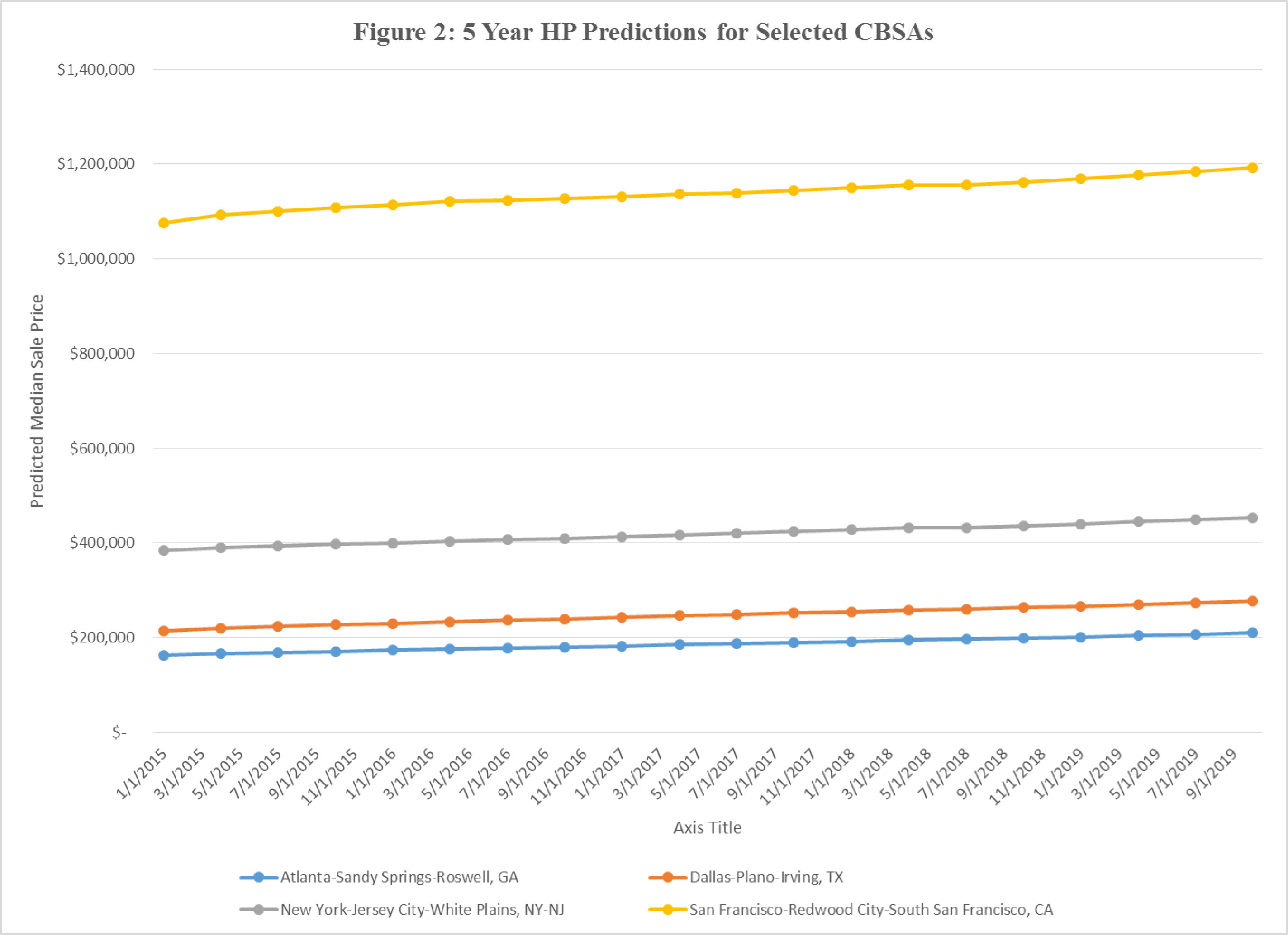
A second exhibit looks at the quarterly predicted MSP for selected CBSAs (Figure 2 above). The predicted levels vary widely among these four CBSAs, as expected. However, they also show similar and modest upward trends. Indeed, the correlation among the predicted values for the five years is quite high. However, as captured in Figure 1, the cumulative changes do vary widely among the CBSAs.
What Are the Key Drivers of the Predictions?
A key question is what drives the cumulative predicted changes in house prices among these 48 large CBSAS. One approach to address this question is to estimate a simple model that explains the cumulative percentage change for each CBSA as a function of the key drivers — the predicted growth in employment and the affordable price and the size of the residual at the beginning of the forecast period (2015:q1). The results of this regression are in Table 2 below.
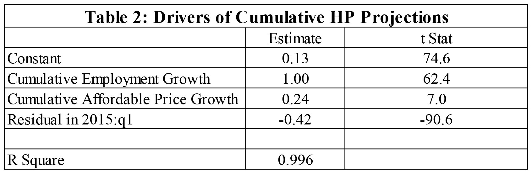
Note, first, that the explanatory power of the simple model is quite high; R2 is 99 percent. Second, predicted employment growth and house price growth grow one for one and the statistical significance of employment growth is quite large. Third, the growth in the affordable price is also significant but quantitatively less important than employment growth. Fourth and most importantly, the impact of the residual is quantitatively large, negative, and statistically significant. This is the key to 2 equation model; that is, CBSAs in which the residual gap is large and positive can expect, all else equal, lower growth rates than places with a small gap. This applies to the three SF Bay Area CBSAs in Figure 1. Likewise, those with relatively large negative gaps can expect relatively fast growth. This is the case with Warren, Michigan and some others with relatively large predicted growth rates.
One great challenge to this interpretation and approach is that the large gap may be representative of very high and realistic expectations of growth in the fundamentals such as employment and household income. That is, the gap may be a little misleading since it does not take into account future expected values of these fundamentals. However, our model tries to address this by basing predictions of employment and the affordable price using CBSA specific trends in these variables. Furthermore, we did some simple tests to see whether historical growth in employment and the affordable price showed a relationship with the residual. No evidence of this was found, hence, our judgment is that the adding the lagged residual to the HP model adds a legitimate and informative piece of information relevant to the predictions of house prices and confirms the thinking expressed in our previous article on bubbles.
The simple regression also provides an opportunity to adjust the predictions based upon alternative views about the growth in employment and the affordable price. For example, adjusting the employment growth rate for, say, San Francisco by 30 percent (6 percent per year) would increase the predicted cumulative price change from 24 to 27 percent. Other sensitivity analysis of this type could be performed for other places and with the affordable price.
[i] The variables are entered as the natural logarithms of the variables; for example, the natural log of the median sale price (lnMSP) is the dependent variable in the first equation and dlnMSP is the dependent variable in the second equation.
[ii] This is the approach used by J. Follain and S. Giertz (2013) in their report for the Lincoln Institute of Land Policy entitled “Preventing House Price Bubbles”, which is available at: https://www.lincolninst.edu/pubs/2245_Preventing-House-Price-Bubbles.