By James R. Follain and Michael Sklarz
Collateral Analytics recently announced a new product: a Credit Risk Model. The model is designed to measure the credit risk associated with residential mortgages. Credit risk stems from the potential default by mortgage borrowers. A key goal of the model is to highlight variations in the credit risk among housing markets.
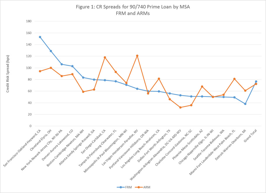
The central output of the model is the credit risk spread (CRS), which measures the annualized cost of mortgage default over the life of the mortgage. Figure 1 provides an example of the distribution of the CRS for 20 large CBSAs. These are based upon a mortgage with a 90 percent LTV and a 740 credit score and are calculated separately for fixed rate (FRM) and adjustable rate (ARM) mortgages. In this example, the largest CRS for the FRMs are in San Francisco (153 bps) and Cleveland (129 bps); the largest for the ARMs are for San Diego (118 bps) and Las Vegas (121 bps). The CBSA with the smallest CRS for the FRM is Detroit (38 bps); Charlotte and Washington DC are at the bottom for ARMs at 36 and 32 bps, respectively. There is wide variation around the average values of the CRS, which are 77 bps for the FRMs and 73 for the ARMs, as such, they confirm a central assumption underlying the CA CR Model – credit risk varies widely among local housing markets.
An obvious an important question is this: what drives these variations? Three categories of factors drive the values of the CRS. One is the set of equations that predict the probability of default and prepayment. Our model estimates these equations separately for 20 large CBSAs and some of the MSA Divisions within them. Another is the house price scenarios that are fed into the default and prepayment equations. These also vary by MSA. The final set of factors are those that determine the losses given a default (LGD). These include the REO Discount and the number of days typically needed to complete a foreclosure. The REO discounts are generated by CA and can vary down to the zip code level.
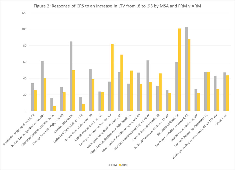
Sorting out the specific roles that each of these three factors in generating the CRS is a complex undertaking. This is especially true for the first factor – the default and prepayment equations, which consist of 50 plus coefficient estimates in the two equations. In this article, we offer a summary measure of the effect of the coefficient estimates. We compute the change in the CRS by MSA for an increase in the LTV from 80 to 95 percent. In this calculation, everything is held constant accept the processing of the HP scenarios by the equations. These are summarized in Figure 2. The largest impacts of a change in the LTV from 80 to 95 percent on the CRS for ARMs are in Las Vegas (82 bps), San Diego (101 bps), and San Francisco (88 bps); the smallest CRS for ARMs are in Washington (27), Detroit (23), and Atlanta (26). San Francisco and Cleveland top the list for FRMs and Seattle, Charlotte, and Dallas are at the low end of the range for FRMs. Again, the variation in the impact of the equations on the CRS around the average is considerable and consistent with our efforts to measure them.
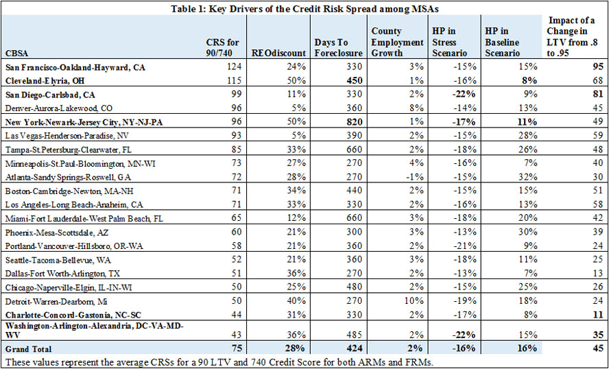
We now combine this information about the impact of the equations on the CRS with other drivers of the CRS that vary among markets to highlight features of the CBSAs that are associated with relatively large and small CR spreads. These additional factors include the REO Discount, the average days to foreclosure, the county employment growth rate, and the stress and baseline HP scenarios. These are contained in Table 1 and the CBSAs are ranked from those with the highest average CRS to the lowest; these are the averages for a 90/740 loan and are averages for the ARM and FRM.
San Francisco, which has the highest CRS, is also the CBSA in which the equations play the largest role; a 15 percent increase in the LTV from 80 to 95 percent increases the CRS by 95 basis points compared to an average shock value among all CBSAs of 45 bps. The other drivers of the CRS for San Francisco are not far from the average values for all CBSAs. San Diego is another CBSA near the top of the list in terms of the CRS in which the equations play a key role, i.e. the shock value is 81 bps. Cleveland is also near the top of the list in terms of the CRS but other factors underlie its ranking. In particular, its baseline HP is below average and its stress scenario above average; also, the days to foreclosure and the REO Discount for Cleveland are also well above average. At the bottom on the list are Charlotte and Washington DC, where the shock values are quite small.
In sum, the CA Credit Risk Model accomplishes a key goal – highlight variations in credit risk among markets. Though providing definitive explanations for the variations is a challenge owing to the complexity of the model and, more fundamentally, the wide range of factors that affect credit risk, it also provides insights about why the CRS varies among markets. A key factor seems to be the default and prepayment equations and their sensitivity to shocks in house prices. As such, this supports our view that estimates of these equations at the MSA or CBSA level can yield important insights about the variations in the CRS among markets.
Download a PDF file of this research paper here.