New Forecasts of House Prices at the MSA Level

by Dr. James R. Follain and Dr. Michael Sklarz

Five Year Forecasts of House Prices: A New Product from Collateral Analytics

An important stylized fact of US housing markets is that movements in the price of housing can vary widely among local housing markets. A recent article which appeared on the Collateral Analytics website entitled “Here is Strong Proof of Wide Differences in Local House Prices” by Follain and Sklarz (2014) highlights this point. An implication of this stylized fact is that movements in future house prices will continue to vary widely among markets. The challenge is predicting what these changes might be.  It is surely well-understood that predicting future house price movements is not an exact science, but a wide variety of evidence does suggest that econometric models can shed light on what those movements will be.

The primary purpose of this article is to introduce a new model of house prices at the Metropolitan Statistical Area (MSA) level by Collateral Analytics. The model forecasts future house prices for 384 MSAs for a five year period: 2014:Q3 through 2019:Q2. A longer article on the CA web site provides more details about the estimates of the model, its predictive power, and a variety of other measures of the model forecasts. Here focus is upon a brief summary of the model and one set of forecasts.

Description of the CA House Price Model and Key Assumptions Underlying the Model

The model consists of a single equation that is estimated separately for nine groups of MSAs. The dependent variable is the natural log of the median sales price. The drivers of this measure of house prices include the lagged values of employment, household income, and the number of households, all of which are measured in natural logs. Two interest rate measures are also included: the level of the 10 year Treasury Bond and the gap between the 10 year and 1 year Treasury rates. The final variable in the model is the index of US House Prices, as measured by FHFA’s repeat sales index. The estimated equation also includes MSA specific fixed effects, which capture the average gap between the level of prices in an MSA and the amount predicted by the economic variables in the model. Quarterly data from 1984 through to 2014:q2 and 384 MSAs are used for the estimation.

A key assumption of the new model is that is that it is best estimated by pooling groups of MSAs. This is an intermediate approach between two extremes. One extreme would pool all MSAs and generate a common set of coefficient estimates for all MSAs in the U.S. This runs the risk of imposing inappropriate coefficients for many or most MSAs. The other extreme is one in which the model is estimated separately for each of the 384 MSAs in the sample. This can result in less precise estimates due to relatively smaller sample size and omitting common ground and known interactions among MSAs. Of course, choosing these groups is a judgment call. Our approach uses nine different groups of MSAs. Three are based upon employment growth between 1990 and 2010 and three are based upon the size of total employment in an MSA in 2000. The groups represent those above the 75^th percentile, below the 25^th percentile, and those between these two percentiles.

The combination of these groupings of MSAs and the estimation procedure provide the opportunity to capture some of the many other traits of a local market that affect house prices but are difficult to measure and incorporate into a model of house prices. For example, some markets are more impacted by international buyers than others, e.g. New York, Miami, San Francisco, Los Angeles, etc. A specific measure of international demand is not incorporated into the model but its impact may be captured in one of two ways in the model. First, the approach generates estimates of what are called MSA fixed effects. These fixed effects measure the persistent departure or gap between the level of house prices in a market and what the fundamental drivers of house prices incorporated into the model.  These fixed effects vary among the 384 MSAs in the sample and can reflect this left out factor. Similarly, the nine groupings of the MSAs include one for the largest MSAs, which allows the model coefficients to capture the influence of some of the potentially left out variables.

The model rests upon the predictions of the underlying variables that drive house prices. The predicted values of the number of households, median household income, and the level of employment at the MSA level are based upon CA’s own forecasts for these series. The interest rate and U.S. house price projections are based upon recent projections of the Federal Reserve Board for its CCAR program.[1]

FORECASTS

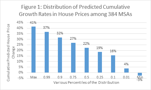
Figure 1 offers a summary of the cumulative predicted house price changes from 2014:q3 through 2019:q2 for the baseline scenario.  The median cumulative price change is 22 percent, which is about 4.5 percent per year. The most optimistic predictions call for 6 percent or more per year. About 10 percent of the MSAs fall into this category. At the other end of the spectrum, 10 percent of the MSAs are projected to grow at 3 percent or less per year. 50 percent of the MSAs are predicted to grow between 19 and 27 percent during the five year forecast period. Palm Coast, FL and St. George, UT top the list with predicted growth rates of 41 and 38 percent, respectively. At the other end of the tail are Albany, GA (0 percent) and Rocky Mount, NC (-3 percent).