Download a PDF file of this research paper here
Introduction
Predicting how long it will take to sell a home depends on a number of factors including the general macro-economic environment. The macro-economic environment would include anything which affects the overall economic outlook, and for residential real estate, mortgage rates and credit access would be at the top of that list. We should also note that there will be different skill levels among real estate agents who are better at staging and marketing a home. Here we focus on three important additional components that help determine how long it will take to sell a home. First, market conditions as reflected by Months of Remaining Inventory. Second, seasonality which takes into account when a home is put on the market. Third, and most relevant, how the home is priced relative to its true market value.
I. Pricing Strategy
The decision on how to price a property for sale is nuanced, has varied over time, market conditions, and across markets. The reason there even exists a pricing strategy is primarily because housing is a complex bundle of goods and services and some homes are more unique than others. Buyers are also unique, possessing different levels of information, relying on different sources of information, some with aligned interests and some that only imply their interests are aligned. Each person will value any given property differently. As a result of different values or reservation prices, a transaction eventually turns into a negotiation between potential buyers and the seller. The starting point of the negotiation is usually the listing price of the property. As with many things in life, the path you take and how you get started can have important implications on the outcome. The discussion below is concerned with the interaction of the listing price and how long it takes to sell the property.
Research has suggested it is not possible to maximize both the selling price and minimize selling time. A lower price relative to market value will generally result in a faster sale, but not necessarily at the highest price. In cases when market conditions are strong and there exist many potential buyers, we have observed that intentionally underpricing a home for sale and encouraging bidding wars will sometimes result in offering prices far above the list price. But this is only true when market conditions are strong. When the potential number of buyers is thin, then a low list price will simply generate lower offers.
Historically, sale prices have been in the mid-90% range figure as a proportion of list price. That is, when a seller asks $500,000 for a home, the typical final sale price is $475,000 to $490,000 and it sells within a reasonable time on the market, similar to other homes in the neighborhood. If the true value of the home were in the range of $475,000 to $490,000 then we would find such a result reasonable, and in line with expectations. But what if the home was actually worth $450,000 or $550,000, then how would this affect the expected time to sell? We explore this question below, after reviewing how market conditions and seasonality affect the average time on the market.
II. Market Conditions and Time on the Market
The time on the market is, almost by definition, related to market conditions. When the supply of housing is fixed or increasing slowly and demand is increasing (due to fundamentals or the availability of credit) we should expect increasing prices, bidding wars and typical homes selling quickly. In contrast, when demand is declining and supply is fixed or over-built then prices should decline.
There are many other nuances that change the time on the market over the business cycle and Case and Shiller (1988) find that home buyers in boom cities had much higher expectations for future price increases. That is, buyers assumed recent past year price increases would continue. Such buyers were also more influenced by investment motives versus consumption motives. There is evidence of anchoring from the recent past for sellers as well. Case and Shiller found excess demand in boom markets and excess supply in the post-boom market. Boom markets, with rapidly increasing prices, could occur because of declining interest rates or strong economic growth relative to supply. In such markets, time on the market declines. When the economy is slowing, and interest rates increasing, prices will slowly increase or decline, while time on the market increases.
In 2015, Collateral Analytics developed a set of more localized market condition indicators that could affect price or days on market. Among these, for the prior year, are:
- Number of Sales
- Absorption Rate
- Number of Active Listings
- Months of Inventory Remaining
- Median Sold Price
- Median Sold Market Time
- Median Active Listing Price
- Median Listing Active Market Time
- Median Sold-To-List Price Ratio
- Number of Foreclosure Sales as a Percentage of Regular and REO Sales
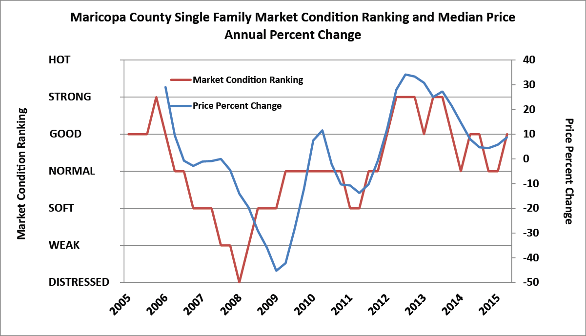
Markets have since been graded from distressed to hot, based on seven categories. Most of the time, markets are in good or normal ranges. In 2009 and 2010, most markets were soft or distressed, and in 2006 most markets were strong or hot. An example of one county market, Maricopa (Phoenix) is shown below in Exhibit 1 with market conditions shown over time. We see the market condition rating in red and the price changes in blue. The data shown is simultaneous with no leads or lags. Generally, we see market conditions leading price changes, but that lead seems to be decreasing over the years.
Exhibit 1: Market Conditions Vary Over Time
Market conditions are continuously graded by zip code for the entire US and this data is fed into our empirical analysis for estimating time on the market. One of the more prominent indicators of market conditions, Months of Remaining Inventory, is further explored below in section four, but first, we must point out the role of seasonality, seldom controlled by most of the prior literature or practitioners, in terms of impact on time to sell.
III. Seasonality and Time on the Market
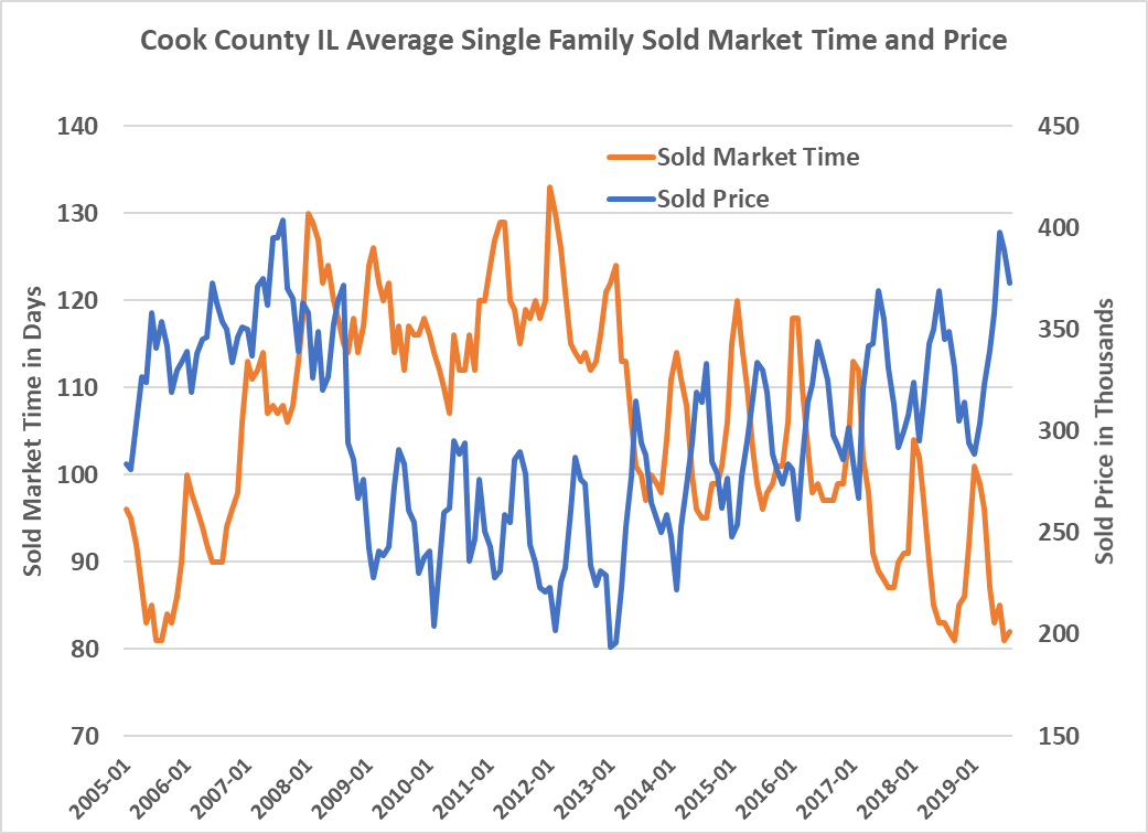
Sales of homes peak at different times of the year across the country, and many commonly known factors affect these cycles like school patterns, employment patterns, holidays and weather. While the pattern of sales over the course of a year is common knowledge among real estate agents, few appraisers explicitly consider the time of year a home is listed for sale. Our research has previously shown that not only do sales volumes vary over the course of a year, but so do sales prices, with higher prices during the peak spring/summer months and lower prices in the softer late fall/winter period. Exhibit 2 shows monthly single family sold prices for Cook County IL (Chicago) along with sold market times. Note the clear inverse relationship between the two as well as the seasonality with respect to sales volume.
Exhibit 2: Seasonality of Sold Prices and Sold Market Times
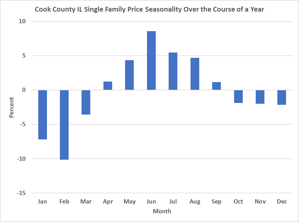
There is also seasonality with respect to prices and we can see this in Exhibit 3, based on historical Chicago patterns for the last ten years by examining the relative sales prices per square foot for similar properties over the course of each year. Homes that close in February are typically sold at prices some 10% below the average for the year, while homes that close in June or July run 8% above average.
The worst possible listing time would be around Thanksgiving in the late fall where your home could possibly sit until buyer activity accelerates in the spring. For example, the same Chicago area home, that is fairly priced, might take six months to sell if listed late in the year, and only two months to sell, if listed in May.
Exhibit 3: Typical Price Deviation in Cook County (Chicago) for Residential Property
If homeowners wished to maximize investment gains, they would certainly sell during the peak months and purchase during the troughs. Unfortunately for most homeowners, the decision to move often creates the need for both selling and buying, lest the homeowners decide to temporarily rent and move twice, adding significant transaction costs to the move and negating much of the benefits from timing the purchase and sale. To the extent these moving costs are significant, the variations in price observed here over the course of the year are rational and explainable. Still, it does allow for some exploitation by first-time buyers or last-time sellers as well as speculators in the housing market.
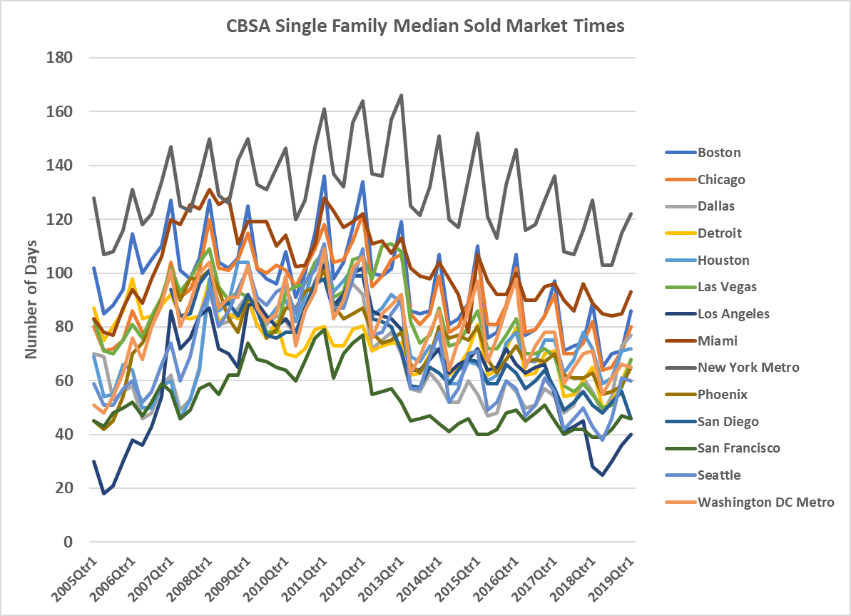
Seasonality exists in all markets, even those where climate varies less than Chicago. Seasonality can be observed in Exhibit 4 shown below which shows the median days on market (DOM) for all quarters over a number of years. We see the consistent pattern of longer DOM for properties put on the market in late fall or winter. In 2009 we see a large number of faster sales as a result of foreclosures and quicker bank REO sales. Generally, we see markets slowing from 2005 through 2011 and then returning to normality and even quickening over time. Whether this decline in DOM will continue is difficult to say, but a general lack of inventory and slightly lower volumes is consistent with this faster sales trend seen in recent years. Reasonably priced homes generally sell within 90 days, with the current typical range of 60 to 80.
Exhibit 4: Median Sold DOM Over Time for Major CBSAs
IV. Months Remaining Inventory, MRI, by Price Range
Among the market conditions indicators, one is dominant. It is Months of Remaining Inventory or MRI. Generally, markets with three or fewer months of inventory are strong or hot. Those with four to six months are fairly normal, while those with more than six months are softer. But we do see that what is normal also varies by price range and we show that below.
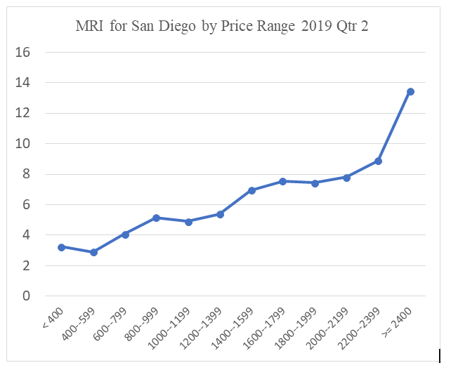
We show below three exhibits that represent typical patterns of increasing months remaining inventory by price range, for Cincinnati, Columbus (OH), and Indianapolis, with additional exhibits for Atlanta and San Diego below. Generally, the higher the price range within a given market, the more time is required to sell and most often, the months remaining inventory will be higher. Stated another way, relatively higher priced homes, within the same market, are usually thinner (less liquid) markets requiring more time to sell.
Exhibit 5: Months Remaining Inventory for Three Midwest CBSAs

Exhibit 6: Months Remaining Inventory for Atlanta CBSA
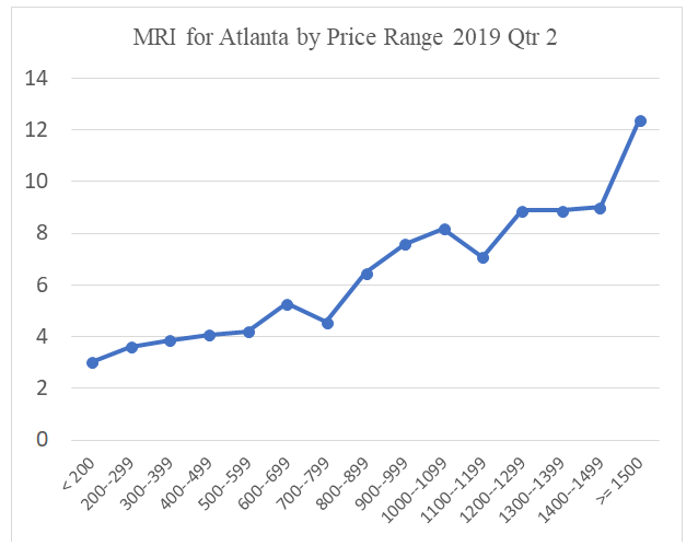
Exhibit 7: Months Remaining Inventory for San Diego CBSA
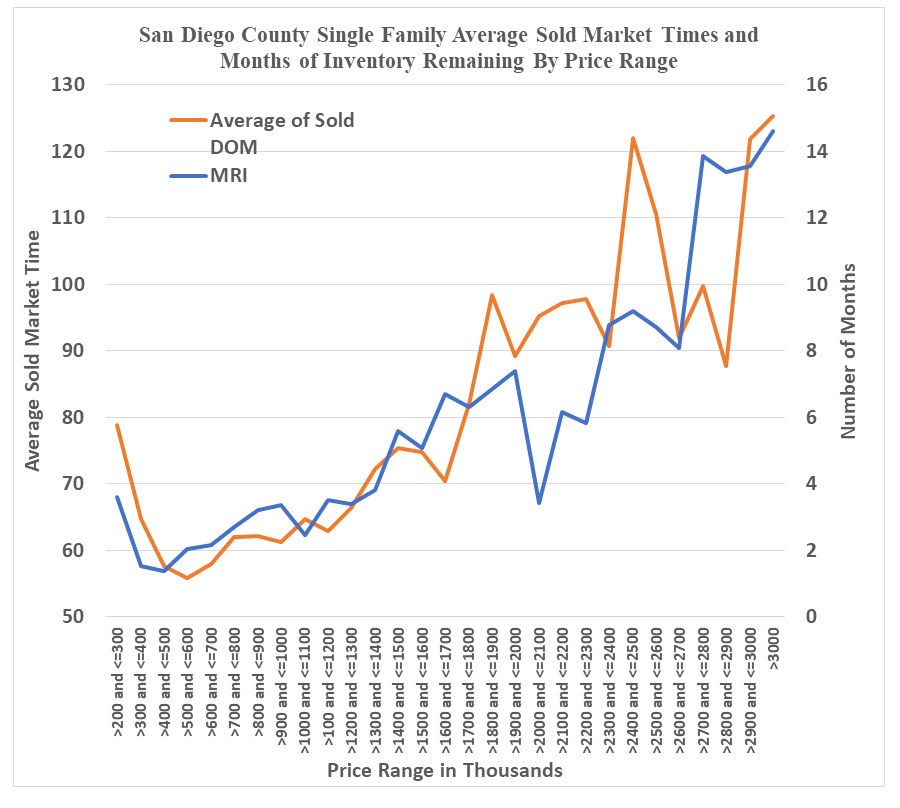
Below we combine the MRI with price ranges and DOM. In Exhibit 8, we show this relationship over the 57 quarters from 2005 through the first quarter of 2019, broken into price ranges for San Diego. This is a typical graph, where the very lowest price tiers (bottom 3%) generally take longer to sell. Examining the types of listings in this bottom price range and you will find “mobile” homes on leased land sites, and properties with various title defects. Generally, we observe higher MRI and longer time required to sell a home as the price tier increases, the market thins, and the properties become more unique.
Exhibit 8: MRI and DOM for Price Tiers Over 2005, Qtr. through Qtr. 1, 2019
V. Pricing Relative to Market Value
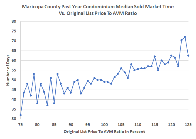
Using the Collateral Analytics Automated Valuation Model (CA Value AVM) for the estimate of market value, we can compare the list price of homes with these values in the form of a ratio with the expectation that the lower the list price to AVM the faster will be the sale. Note that even homes that sell in a few days will appear to have required at least 20 to 30 days, as it takes time to arrange closings. Below in Exhibit 9, we show the average single-family DOM versus the ratio of the original List Price to the AVM for one sample market, Phoenix using the most recent year of data. We also show the same relationship for condominiums in Exhibit 10. Homes and condos priced higher relative to market values can take considerably longer to sell. In both exhibits, the 100 mark is where our estimate of value equals the list price. When one considers that there is a fixed time period required prior to closing, the difference in time required from listing to contract agreement is even more significant than may appear below. It is true that market values are highly correlated with list prices, but it is also true that some sellers and their agents are more optimistic on the value of their home/listing and we see this relative pricing as a very significant driver of how long it takes to sell a home. Shown below are those homes which sold successfully. Keep in mind that a large portion of the overpriced homes simply expire without selling. Sellers that ask such high prices, relative to true market value, may be in fishing mode only willing to sell if someone pays a relatively high price. Such sellers are also not very motivated, while those asking lower prices relative to value are motivated and we see this in the faster average selling time.
Exhibit 9: Impact of Relative List Price/Market Value CA AVM Estimate on Time to Sell Using Phoenix as an Example

Exhibit 10: Impact of Relative List Price/Market Value CA AVM Estimate on Time to Sell Using Phoenix Condos as an Example
VI. Conclusions
It is not possible to sell at a relatively high price and in a relatively short period of time without a lot of luck. Reasonably priced homes will typically sell in 30 to 80 days, with many selling faster, especially if listed in spring and early summer months. It is not unusual to see a home sell within 30 days today as many markets simply lack inventory, especially for any home in the bottom half of the price tiers within a given metro. As of late 2019, homeowners are sitting on low mortgage rates and reluctant to upgrade during an uncertain economic outlook. In markets like California, Proposition 13 also reduces the turnover of property and impacts the lack of supply of existing resale homes on the market.
Generally, relatively higher priced homes within any given metro, take longer to sell, sometimes by a significant margin as these markets tend to be thinner.
Asking price relative to market value matters a great deal. Our research suggests that typical list price to selling price ratios run 95% to 105% and being within 5% of true market value is necessary to not deter potential buyers. Homes listed at 110% of market value, or higher, can take considerably more time to sell. At the same time, bidding wars may occur on some underpriced homes, resulting in selling prices above asking prices, but only in good to strong markets, so this is a risky strategy unless the market is strong.
Seasonality also matters a great deal, as do market conditions, reflected by Months of Remaining Inventory. These are observable for any market and price range making days on market quite predictable, particularly when selecting an experienced and well-connected real estate agent. Sellers that wish the shortest days on market will put homes on the market in the spring and generally try and avoid weak, soft or distressed markets to the extent possible. This can be monitored by watching market conditions over time, especially the key Months of Remaining Inventory indicator.
References
Case, K. and R. Shiller 1988, The Behavior of Buyers in Boom and Post-boom Markets, NBER Working paper no. 2748, Oct. 1988.
Knight, J. R. 2002. Listing Price, Time on Market, and Ultimate Selling Price: Causes and Effects of Listing Price Changes. Real Estate Economics 30 (2), 213-237.
Merlo, A., & Ortalo-Magne, F. 2004. Bargaining over residential real estate: evidence from England. Journal of Urban Economics 56, 192-216.
Merlo, A. F. Ortalo-Magne, & J. Rust, “The Home Selling Problem: Theory and Evidence”, PIER Working Paper 13-006, http://ssrn.com/abstract=2209103, Jan. 2013.
Miller, N. G. Time on the Market and Selling Price. American Real Estate and Urban Economics Association Journal (Real Estate Economics) 6 (Summer 1978), 64-73.
Miller, N.G., V. Sah, M. Sklarz, and S. Pampulov “Is there Seasonality in Home Prices – Evidence from CBSAs”, Journal of Housing Research, Vol. 22, No. 1, pp 1-17, 2012.
Miller, N. G. and M. Sklarz “Pricing Strategies and Residential Property Selling Prices,” with Michael A. Sklarz, The Journal of Real Estate Research. Vol. 2, No. 1, Fall, 1987.
Miller, N. G. and M. Sklarz “Leading Indicators of Housing Market Price Trends,” The Journal of Real Estate Research, Vol. 1 No. 1 Fall, 1986.