by Dr. Michael Sklarz*, Dr. Norman Miller** and Anthony Pennington-Cross*** | December 4, 2018
Download a PDF file of this research paper here.
Introduction
Some housing market observers have noticed that higher priced homes, on average, are taking much longer to sell than median priced homes in a number of the nation’s real estate markets. This is not new, nor is it unusual. Perhaps the availability of such data is new to some market observers, but we have tracked Months Remaining Inventory, MRI, for a long time and here we put it into context as one of the many leading indicators of housing price trends that we have examined many times in our prior research.
Default rates on mortgage loans are driven by a number of factors, including but not limited to the following:
- Income to mortgage payment ratio
- Credit behavior and attitudes toward paying obligations as reflected in credit scores
- Loss of a job or unexpected medical expense
- Available liquid assets that may be tapped for mortgage payments
- Perceived and/or actual equity in the home as reflected in current values
While all of the above are important, the last factor seems to dominate all the others. Home equity is a function of current market value and the loan-to-value (LTV) ratio of the original mortgage, along with any other debt added during ownership, such as second mortgages and home equity lines of credit, (HELOC). Here we focus on this last factor, home equity.
When home values decline to the point where borrowers have no equity or negative equity, and they see no immediate reversal in local price trends, they often decide to default. This is sometimes called “rational default” or “strategic default”, and while it may affect credit ratings for some time, US borrowers know they will seldom be chased for mortgage balance deficiencies. This encourages the decision to default when the mortgage balance appears to exceed the value of the home. This creates a situation where mortgage lenders are on the short end of a “heads I win, tails you lose situation”. If prices go up, borrowers’ benefit, but if prices go down too far, the mortgage lender suffers.
The tendency towards default may be reinforced when borrowers know it will take several months to evict them from the home, and meanwhile they can live rent free, extracting more capital from mortgage investors.[1] Some borrowers use the excuse that lenders have misled them or charged too high of a rate, allowing rationalization for not making their mortgage payments.
Below, we illustrate the typical pattern of mortgage default in response to negative price trends and high LTV mortgages, using Chula Vista, CA as an example. These series are based upon Non-Agency RMBS mortgage performance data. Then we compare several local markets, by zip code, where average LTVs and the use of mortgages varies systematically. Last, we show a map of zip codes with default rates. All of these illustrations, while set in San Diego county, are not unique. They are typical of all housing markets where prices have changed significantly.
Chula Vista: A Market with Higher than Average LTV Mortgage loans
In Exhibit 1 we see the effects of both high LTV mortgages and significant price swings. Loans originated in the years 2000, 2001, 2002, and 2003 were the beneficiaries of strong price increases of 12%, 14% and 25% in average home prices, so when prices reversed in 2006 there was still sufficient cushion to preserve real home equity. Independent of factors 1 through 4 above that influence default, factor 5, home equity was sufficient that few home owners defaulted. Note that during this period of time the average purchase mortgage LTV was climbing every year, as shown in Exhibit 2. Mortgage loans originated in 2004 saw increasing default rates peaking out in 2007 as home prices started to decline in 2006. Loans originated in 2005, 2006 and 2007 at the peak of home prices in the cycle, and cumulatively half or more defaulted in the subsequent years. The high LTV loans declined as subprime loans disappeared, however, the FHA and loan modifications allowed many home owners to continue with high LTVs through 2012.
Exhibit 1 Chula Vista Zip 91913 Default Rates by Year of Origination
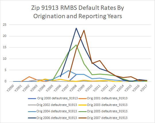
Exhibit 2 Chula Vista Zip 91913 LTV by Year

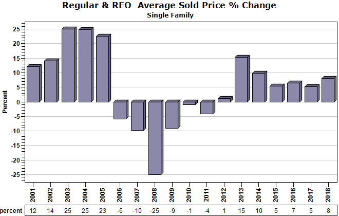
In Exhibit 3 we show the annual average percentage change in price by year in Chula Vista. Prices increased rapidly as mortgage credit became easier in the 2003 through 2005 period, then fell as easy mortgage credit reversed. Those who were late in following the herd of home buying enthusiasts, often paid prices that were unsustainable with current household income. Modest home price appreciation, closer to inflation and wage growth, is sustainable, but we see the market overshoot and undershoot these more sustainable levels.
Exhibit 3 Chula Vista Zip 91913 Price Percent Change Trends
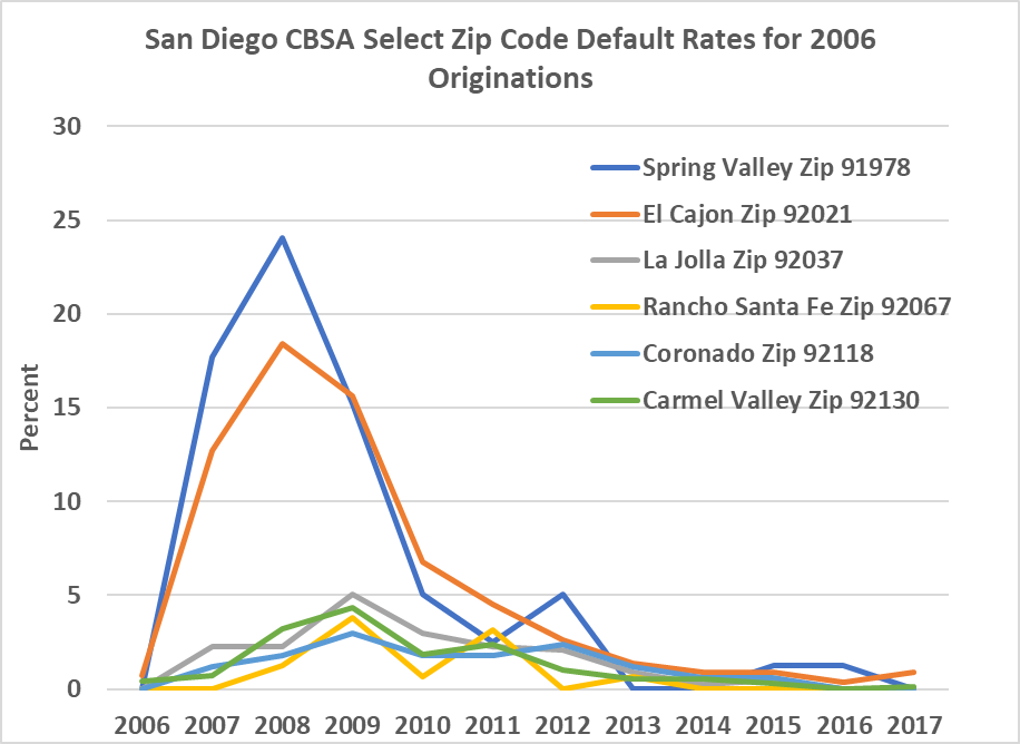
To expand our analysis, a range of markets were selected from the same county, where we see significantly different levels of original mortgage leverage. Below are six markets, with average mortgage LTVs for the combined years of 2005 and 2006, shown in the first column and in the second column are the percentage of transactions during 2005 and 2006 where no mortgage is used at all. This is significant as an indicator of contagion from the local market. Areas with all equity homes tend to be more stable with fewer foreclosures. The lower the rate of foreclosures, the fewer “distressed” sales that might be used by appraisers or buyers as indicators of value for any local property.
| Average LTV % 2005 & 2006 | Percentage with No Mortgage | ||
| 91978 | Spring Valley | 92 | 9 |
| 92021 | El Cajon | 89 | 8 |
| 92130 | Carmel Valley | 73 | 8 |
| 92118 | Coronado | 73 | 21 |
| 92037 | La Jolla | 69 | 17 |
| 92067 | Rancho Sante Fe | 69 | 29 |
Next, we combine all of these markets in two Exhibits, 4 and 5, comparing default rates for loans originated during the peak of easy credit, 2005 and 2006. What we observe is that those markets with higher LTV mortgages and similar price trends as Chula Vista, defaulted at much higher rates. It is very clear from these patterns that home price trends dominate the decision of home borrowers to default. Price declines in 2008 were especially influential in that most borrowers expected these negative trends to continue.[2]
Exhibit 4 Six Zip Codes and Mortgage Default Rates for Loans Originated in 2005
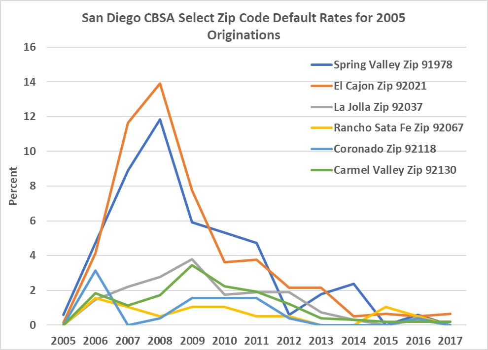
Exhibit 5 Six Zip Codes and Mortgage Default Rates for Loans Originated in 2006
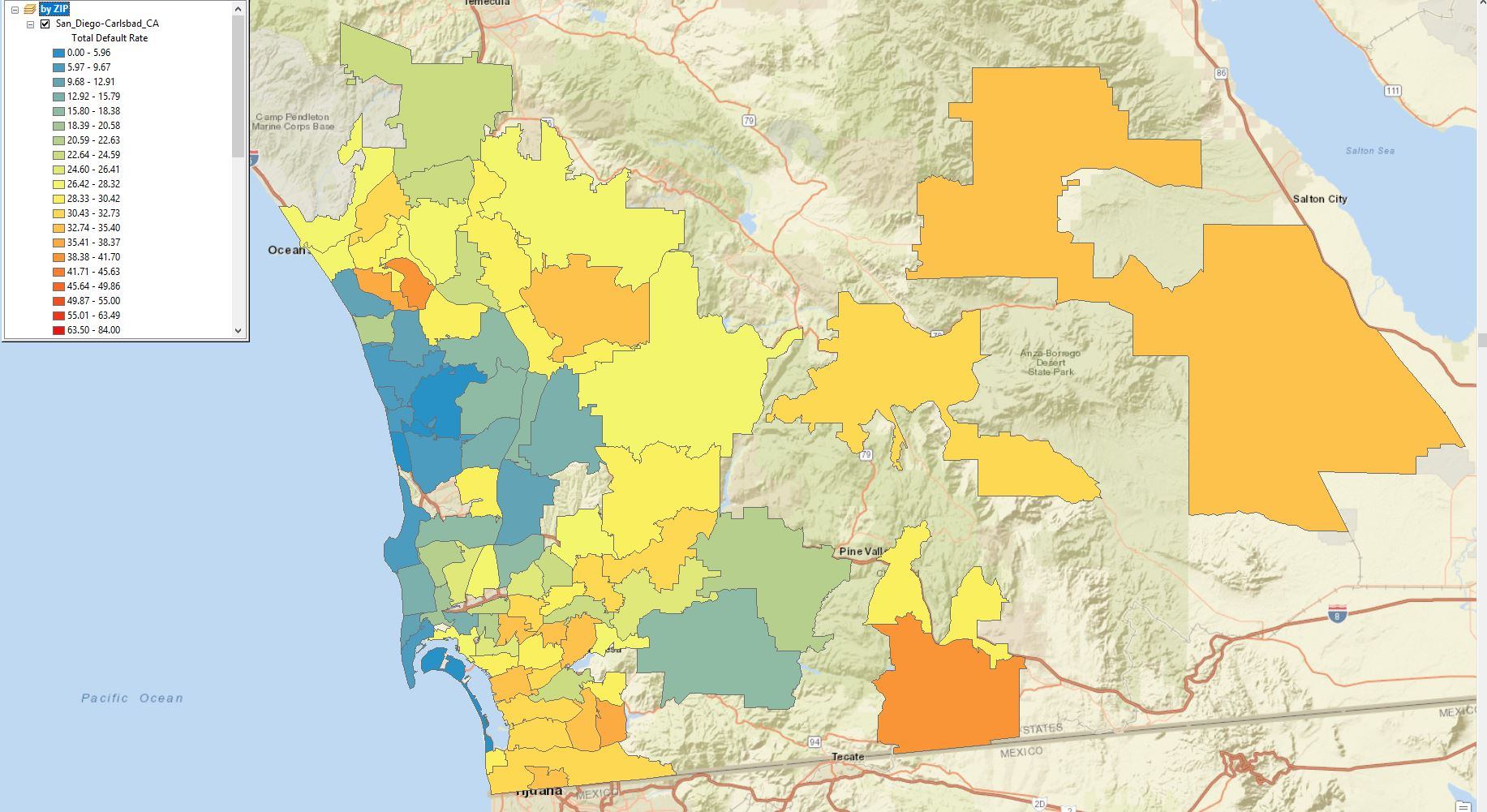
Last, we show a map of many zip codes in San Diego and default rates for all mortgages originated from 2000 through 2007. The areas in darker blue have the lowest default rates. These are areas where mortgages are less relied upon and LTVs tend to be lower. The yellow and orange colored areas are neighborhoods where home buyers have less access to wealth for down payments, use higher LTV mortgages and thus are more apt to go into financial stress should home prices decline. The math is quite simple. If the average LTV was 92% in a local market and home prices slip just 8%, that home equity is wiped out. Add in transactions and legal costs and we can see that mortgage investors are very vulnerable. In previous articles we have discussed how mortgage investors and in turn, lenders, could deal with these price induced risks. They need to account for not only current values, but also price uncertainty and future price trends. This is certainly possible by adjusting LTVs to a statistically driven range of confidence.[3]
Exhibit 6: Default Rates by Zip Code for San Diego
Conclusions
We are not suggesting any sort of neighborhood level, absolute screening for mortgage underwriting criteria. We are suggesting that price uncertainty and actual and expected equity are extremely important drivers of mortgage default. Thus, good valuation models with information about price uncertainty and even price forecasts are factors that should be considered by mortgage investors.
*Collateral Analytics CEO
**University of San Diego School of Business and Collateral Analytics Research
***Marquette University College of Business and Collateral Analytics Research
Footnotes
[1] State laws and the borrower’s rights after default vary considerably by state, which in turn affects borrower behavior. For example, see “Recourse and Residential Mortgage Default: Evidence from US States” by A. Ghent and M. Kudlyak in The Review of Financial Studies, Volume 24, Issue 9, 1 September 2011, Pages 3139–3186.
[2] In many surveys by Case and Schiller of home owners, asking what next years home appreciation rate will be, the typical answer was whatever happened in the most recent year.
[3] See our previous paper on adjusting loan quality to price uncertainty, by considering for example, the 80% confident lowest possible price instead of simply using average value estimates. More sophisticated analysis might even use the lowest price expected over the next three years when mortgage risk and default historically peak out.