by Michael Sklarz, Ph.D., Jim Follain Ph.D., and Norm Miller Ph.D.
A strong desire exists among home owners, mortgage lenders, and others with key stakes in the housing and mortgage market to better understand the future direction of house prices. Indeed, Collateral Analytics, hereafter CA, and others have built models of house prices and use them to make forecasts of the future. The CA HomePriceTrends analytic platform product includes one set of our estimates. CA’s Credit Risk Model also incorporates five year predictions of house prices at the metro area. These include a baseline scenario and six alternative scenarios around the baseline. Such variation is critical to an understanding of the credit risk inherent in mortgage lending. A number of articles are on the CA web site about these and other models of house price growth. A recent one demonstrates that the growth in house prices is negatively related to the gap between the current level of prices and the level predicted by long run fundamentals such as employment and the affordable price.[1]
There are a number of common themes in these articles and models. First, while acknowledging the challenges of predicting future price movements, the analysis strongly supports the idea that we do, in fact, know something about where prices may go in the future. Second, it is important to highlight the role of local market conditions in any model of house prices since these capture the “alpha” component in house price growth. Third, it is important to continue the process of model development and, especially, take advantage of new sources of data and information about local housing markets.
With this in mind, we offer a new version of the CA House Price Model in this article that builds upon the existing model and incorporate new data. The model incorporates two major changes. One is that the model is estimated at the county level, which offers the opportunity to take a more geographically granular look at the drivers of house prices than one based upon metropolitan areas, states, or the nation. The second is that the model is now estimated with a set of variables that includes both long-run and short-run drivers of house prices. The long-run drivers include local area employment, wages, and mortgage interest rates. Over the long-run, increases in local employment and income and decreases in the mortgage interest rate are positively correlated with house price growth. The short-run drivers or local market conditions include a number of measures of activity in the sales of single family properties such as the number of listings, the months of remaining inventory, and others. In aggregate form, “the CA Market Conditions Index (MCIndex)” reflects several highly correlated market conditions in a single variable. This measurement index was recently discussed in an article on the CA web site.[2]
Brief Summary of the Model
The model consists of two equations. The first explains the level of house prices on a quarterly basis (per quarter) from 2005:q1 through 2014:q4 for each of the 201 counties in the sample. House prices are measured by the natural logarithm of median sales price per square foot for that market and time period. We use median price per square foot since, in contrast to the median price, it normalizes the sold price for different size homes. This equation focuses upon the long-run drivers, which include the level of employment, the affordable price, the national HP index, and year dummy variables (0 or 1). The data are estimated by pooling each of the counties and the models incorporate county fixed effects. This equation is used to construct the gap or the residual between the level of prices and the level predicted by this equation.
The second equation focuses upon the change in the price per square foot. One key driver is the lagged residual from the first equation. All else equal, the larger this gap, the slower house price growth is expected to be as prices are seen as having overshot their long-run or sustainable levels. The other set of drivers includes measures of short-run market conditions such as the turnover rate (number of sales divided by the number of SF housing units in the county), the number of active listings, the ratio of foreclosure sales to regular sales, and the MC Index, which enters as a set of indicator variables scaled from 1 (distressed) to 7 (hot). For example, a lower turnover rate, a higher number of listings and a higher ratio of foreclosure sales are expected to reduce the growth in house prices. Increases in the MC Index are expected to positively impact house price growth.
Data and Filtering
The data used for the estimation of the model come from two main sources. The employment and income data come from the Quarterly Census of Employment and Wages. Interest rates are the 30 year fixed rate mortgage and the national house price index from FHFA. MLS data are used to measure the MC Index and the components included in the model such as the number of active listings and the ratio of foreclosure sales to regular and reo sales. The turnover rate is the ratio of the number of sales (MLS variable) divided by the inventory of single family residential properties, which is generated by CA from property assessor data.
The MLS data are available for over 2,700 counties. A variety of specific criteria are used to select the 201 counties chosen for the model estimation. These include:
- Choose those with data from 2005:q1 through 2014:q4
- Filters to exclude counties with less than 100 sales in any quarter
- Focus on those in relatively large CBSAs
- Filter those with a quarterly price change above 25 percent or less than -25 percent.
The resulting sample consists of data on 8040 observations on 201 counties for the 40 time periods.
Key Results
Table 1 below contains the coefficient estimates for both equations. The first column includes coefficient estimates and other summary information for the first equation (lnMPsqft). The second column contains the information for the second equation (dlnMPsqft). All of the signs of the estimated coefficients are the expected signs and statistically significant. For example, the estimated of the coefficient of the lagged residual (l.hpres) in the second equation is -.11 and has a t statistic of 22, which indicates that increases in the gap between the level of prices and the level predicted by the long run fundamentals tend has a strong and negative impact upon future house price growth. Note too, the strong seasonal pattern in the change in house prices; the second quarter has the highest predicted growth rate, all else equal.
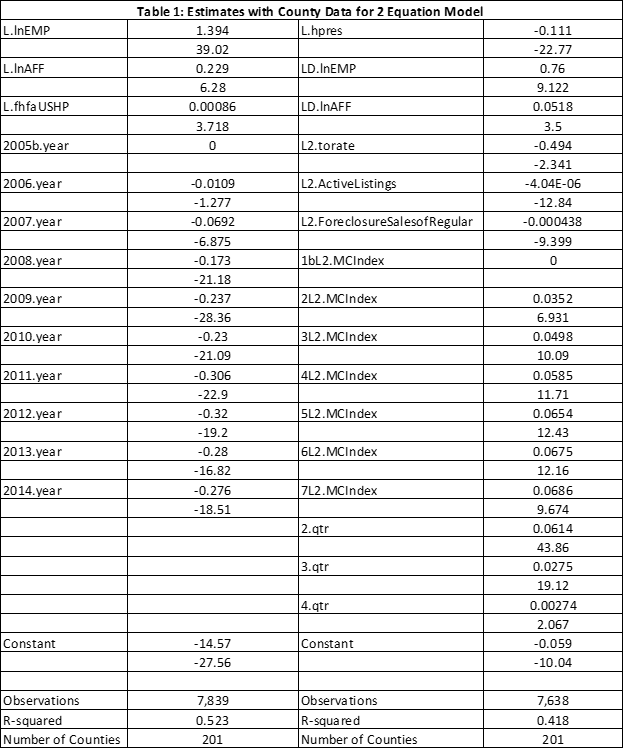
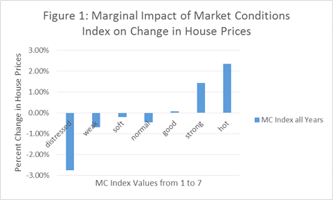
The performance of CA’s MC Index is strong and significant. The estimates of the various indicator variables increase as the MC Index value increases. Another way of highlighting its importance is to examine the change in the predicted growth rate associated with an increase in the MC Index. A summary of this prediction for all years is presented in Figure 1. Predicted growth in the lowest four categories holding all other variables constant is negative, especially in the lowest of the 7 categories (distressed). Predicted growth is substantially positive in the top two categories (strong and hot).
A Look at the Predictive Power of the Model
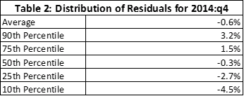
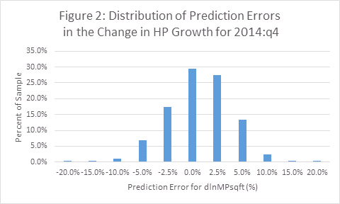
Now we focus upon the errors in the predictions of price changes for one quarter: 2014:q4, the last observation in the data used to estimate the model. The bulk of the errors seem modest as demonstrated by the summary results in Table 2 and the histogram depicted in Figure 2. The overall average error is -.6 of one percent; the median error is -.3 of one percent. 50 percent of the errors are between 1.5 and -2.7 percent (the 75th and 25th percentile values). 80 percent are between 3.2 and -4.5 percent.
However, there are some extreme values of the errors. These are summarized in Table 3 below, which contains the prediction errors of the change in house prices (dlnMPsqft) exceeded plus or minus 10 percent for each quarter of 2014.
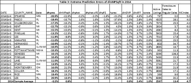
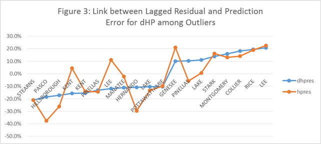
What drives these extreme prediction errors? An examination of the other variables that drive the prediction do not show any major extreme values in the core variables with one exception. That is, the lagged values of the residuals from the first equation are lower among those with relatively large negative errors and vice versa. Figure 3 below seeks to capture this relationship.
We also took a deep dive on one particular county with the largest negative error – Stearns County in the St. Cloud, MN CBSA. Here we noticed a sharp spike in the average number of square feet in a sold home in 2014:q4 of about 16 percent since the previous quarter. This led to a relatively large decrease in the price per square foot. This, in turn, led to a large negative residual for this period, which contributed to a large negative residual for this quarter. This highlights the sensitivity of the results to the oddities or sudden changes in local market conditions that are perhaps not readily captured in the model. One always need to keep an eye out for outlier events to see what the model might be missing.
Final Thoughts and Possible Next Steps
House prices are heavily influenced by local market conditions. These include long-run variables that represent the local employment and household income environment. These also include indicators of the local market for the sales of properties. These also include persistent fixed effects unique to each market. Our latest model demonstrates the importance of including all of these factors. One specific indicator is the new CA index of local market conditions (MC Index), which takes on a value from 1 (distressed) to 7 (hot). The index is compiled from a long list of variables that depict the local real estate market. As expected, a larger value of the MC Index increases future growth in house prices, all else equal. This is a key conclusion of this article and this latest version of a CA House Price model.
An examination of the model predictions for 2014 offers support for the model. The median prediction error of the change in prices is -.3 of one percent in 2014:q4 and 50 percent of the errors are between 1.5 and -2.7 percent. 80 percent are between 3.2 and -4.5 percent. We see this outcome as affirming that house price models offer significant insights about house price movements that can be used to predict the future. Of course, going the next step to make predictions of the future requires predicting the key drivers in the model. Among the most challenging tasks for this purpose is predicting the indicators of the local sales market such as the MC Index and its components. This is the frontier and we are pursuing various approaches so that we can use the model to actually predict future patterns in house prices.
Also, the model does generate some rather extreme errors, both positive and negative. While these are relatively rare, only 6 of the 201 counties had errors above 10 percent or below -10 percent in 2014:q4, they warrant further study. Do these outliers indicate variables that matter but are not included in the model? Or do they represent potential errors or unusual volatility in the data. For example, we find that the average size of a sold property in one outlier increased by over 15 percent in one quarter. We continue to investigate the sources of the errors, but do not at this time offer a “simple” explanation for all of them. Local housing markets are complex. Our model does provide some insights about what drives local housing prices, but they, like models of stock prices, occasionally miss big increases or decreases in prices.
We offer an analogy of how the search for a better model might proceed. CA provides state of the art AVM estimates of properties. We also provide a menu of alternative AVM products that incorporate more information with the goal of increasing the accuracy of the AVM estimate. Something like this may be appropriate for house price models. The base model offers reasonable estimates for most places most of the time, but places with relatively large errors may warrant a more intensive evaluation of local market conditions to see what might have been underlying the error. We will continue the search.
Download a PDF file of this research paper here.
[1] http://collateralanalytics.com/five-year-hp-forecasts-for-large-cbsas-the-key-role-of-the-gap-between-the-level-of-prices-and-the-level-predicted-by-the-fundamentals/. Such a pattern of short term prices oscillation around long terms is not unusual, but here we wish to try and catch those predictors of oscillation to the extent possible.