by Dr. Michael Sklarz and Dr. Norman Miller
Introduction
The very first paper to ever suggest an instrument for hedging residential real estate price risk was entitled “It’s Time for Some Options in Real Estate”.[1] We examined the National Association of REALTORS (NAR) median price index for existing homes, as one possible index that traders could use to hedge or speculate in the housing market, without the need to buy the underlying real estate. The real estate market has always needed an efficient way to go short. Concerns over quantity and quality drift in the sample of homes measured by NAR sales led to a variety of other trading instrument proposals over the years. One novel approach was based on sharing interests in the equity along with the home owner whereby pooled shares were traded for interest in individual home price changes.[2] In May of 2006 an index was offered by the CBOT known as the S&P CS (for the Case Shiller) index. This is been available for about two dozen cities measured at the CBSA level but it has never really caught on. Analysts may wonder why the index has not caught on to the extent expected which begs the question: What do we really want from our indices?
If we want to hedge large national portfolios, then the average for the country as a whole might work. If we want to use the index for hedging a less than evenly stratified portfolio of homes or mortgages, then much more granularity is required. The problem is that even within a single CBSA, prices may be going up in one geographic part of the market and down in another. In fact, if you take the S&P Case Shiller index, discussed below, you will see that a few large movers among localized markets drive the average result.[3]
If we want to know the value of the recently sold and typical home in a given metro then the NAR median price index works fairly well most of the time. But then no one owns the median home in America. The NAR transaction based index provides a good bell weather of general home price trends for new and pre-owned homes. We know it does not accurately measure the average appreciation (or depreciation) for a given home since the average size and quality drifts by market. We know any changes in the composition mix (quantity or quality) in the average home sold in the previous period will distort the NAR Index.[4] As to how representative the NAR data is, based upon the proportion of public record counts sold by Realtors, we can estimate that some 70% or more of all existing home sales are included in the NAR index although they use a subset of these for the index representing 30% to 40% of actual sales.[5] That is a sufficient sample for most indexes, yet the lack of quantity or quality controls for measuring price changes makes this index only a very general indicator of value trends.
The FHFA, (Federal Housing Finance Agency) formerly OFHEO (Office of Federal Housing Enterprise Oversight) uses a weighted repeat sales index that is developed at the CBSA, State and National level. Weighting is based upon the number of sales in each group of housing from the year 2000 so there is some attempt to represent the typical home. They do this by CBSA quarterly and recently started an annual series by ZIP Code at the 5 digit level. [6] The advantage of the repeat sales index approach is that there is an attempt to control for changes in the quality or quantity of the homes represented. Homes may age and wear out over time and so such an index is appropriate for those with a typical home who wish to gauge changes in price. There are two limitations of this index.
First, only conforming loans from Fannie Mae or Freddie Mac transactions are included limiting the sample to those with mortgages under $417,000 as of 2016 with some higher values in select high priced markets. This price limit is sufficient is areas with low density, cheap land and more affordable housing but severely limits the applicability to higher priced markets such as most of California or metro markets like Boston or New York. At the national level homes from expensive markets will be severely under represented.
A second disadvantage of this approach is that repeat sales represent on average only about a fifth of all sales, so most of the sales data is tossed away. In cities with higher stability and low turnover, there will be very little data to use for index construction. In countries like Japan, repeat sales indices such as FHFA’s or Case Shiller’s are totally useless since they represent such a small proportion of the market activity. The smaller the sample, the more noise contained within any price index. Noise can be viewed as the deviations or variance from uncontrolled influences. Larger samples also have noise but the noise cancels out so it is less of a concern.[7]
A third problem with repeat sales indices is that they are subject to transaction bias. Homes that are repeatedly sold may not be representative of the housing stock in general. One study found that houses which sold more frequently appreciated more rapidly than those which did not sell as often.[8] This is no different from stocks which have declined being sold less frequently than those which have appreciated. Home owners are less likely to sell homes that have declined in value.
The S&P Case Shiller’s index approach is also a repeat sales index with the limitations of tossing away the majority of all transactions.[9] The weighting system attempts to hold year 2000 initial sale weights constant so more expensive homes have more weight. Several filters attempt to screen out non-arm’s length transactions and foreclosures but foreclosures that become sold later as REO (real estate owned) by banks are included as repeat sales if they sold more than 12 months since the first sale in the pair. In markets with a lot of foreclosures that become REO sales we will get an unusual and biased price impact on the index. In effect Case Shiller mixes in more distress during downturns which drives the index down faster than if only regular sales were included. Then, after the bottom of a cycle the index will go up faster than if only regular sales were included.[10] In markets with a lot of new homes the S&P CS index will be biased towards older homes which have sold twice and so the index is less representative of the typical home.
One advantage of the Case Shiller index is that they utilize more than simply the conforming loan limit property. Yet, when market trading slows, either seasonally or because of higher mortgage rates and weaker economic conditions, any repeat sales index becomes dependent on thin data which is why it cannot easily be applied to smaller more granular geographic markets. Over short periods of time it is difficult to use a repeat sales based index since there will be fewer recent transactions. Over lapping samples are used to interpolate changes in any given period but these are only approximation techniques.[11] Another disadvantage in the S&P CS index is that changes in the home which influence value including remodeling and additions are often missed. Studies have suggested that these home improvements add a slight positive bias to the repeat sales indices.[12]
If the changes to a physical structure are performed legally, that is, with building permits for modifications, then such modified properties are tossed out. But we know that many home improvements are done without building permits and so distortions in values will no doubt occur. When markets slow down repeat sales techniques using a fraction of the available sales will be subject to greater noise issues and it is not clear how well they hold quality constant, especially in markets with high property taxes where every legal change in the property will result in a higher tax bill.
Because of concerns for thin trading the S&P CS Index is constructed for only larger metro markets. Herein lies another problem. Let’s say you are trying to hedge the localized real estate values or speculate based on condominium prices in the South Loop of Chicago where significant newer and higher quality property has been completed. You may be witnessing prices going up at 4% per year and in order to go long or hedge you want a localized Chicago index but must use an index that includes the vastly different markets of River North or Geneva that may have gone up only 1% over the same period. This much variation between neighborhoods makes localized hedging and speculation less tied to realistic price changes and more tied to a geographically smoothed yet elegant repeat sales model.
Last, the S&P CS index is not fully transparent. A number of filters are used to try and purify the sample. The weighting systems and criteria, such as significant deviations in price from a CS automated valuation model (AVM) estimate of value are inherently black box and difficult to replicate without the assistance of Case Shiller. The market needs transparency and the ability to independently replicate results.
Hedonic pricing models have the advantage of being able to use several times as much data since all sales may be included, repeat or otherwise. Attempts to adjust for quality and quantity changes are based upon regression models that inherently control for these influences. The very best regression models will control for a variety of quantity and quality influences. Yet we find that size (measured by square feet of living area) and age do well to control for quantity and quality, respectively, and often explain more than 80% of the variation in price within local markets. We suggest a strategy based on several indices that can be combined in any manner that reflects a particular portfolio. Imagine a number of geographically localized indices, or property types (condos, single family), or a distressed only index, or homes by size range in tiers from small to large, or by age of home.
When simpler index models are used with fewer property attributes, there is always the concern about quality drift which is why it is sometimes best to draw samples that hold size constant and allow age to match the average age of the existing stock. In other words, there is no perfect index for everyone and bias from uncontrolled effects (noise) will always be a concern, but we can construct a much more accurate picture of property price trends for a specific portfolio or even a single home with a structured sampling approach. The key is simply to slice and dice the data to reflect all manner of price trends. If we wish to reflect the typical home in a given market then we can seek a sample with age in parallel to the local housing stock. Noise may be a problem for shorter time periods with less data, but there are ways to offset this such as using quarterly rather than monthly calculations, or performing a simple smoothing of monthly index values with the Hodrick-Prescott adjustment.[13]
Hedonic models can also be used to develop customized indices or to check for the influence of say foreclosures in a market or simply to run an index on a specific home or pool of homes. This is no different than running a series of AVMs (automated valuation models) for the same home over time.
Which index approach is best?
If current values are of great interest the repeat sales indices do not do very well. The S&P Case Shiller index is reported and produced with a two or three month lag. NAR’s median price index also has a significant time lag along with inconsistencies based on varying degrees of oversight and care by independently managed multiple listing systems.[14] Real estate is one of the few assets we buy that require much time prior to closings necessary to satisfy third parties (appraisers, lenders, inspectors and so forth), so purchase contracts signed in August may close in October and not be reported in an index until December. In the four months since the purchase contract was actually signed, significant changes can occur in market conditions and/or current values. This is why appraisal based models relying on historical data generally lag the market. FHFA and NAR with significant lags will not help if the user seeks an early warning system for market turns. The NAR median price index works well enough in a historical context but should not be relied upon for short term trends and also under represents the lowest priced markets where REALTORs are less involved in the transactions. While the S&P Case Shiller index is a little better, it still lags the market and suffers from sample mix biases.
We suggest a variety of indices that can be customized for each user as well as a series of indices that are publicly disseminated.[15] Below in Exhibit 1, we show that a simple index like price per square foot will generally mirror the more complex S&P Case Shiller index, and it has the advantage of being available two to three month’s sooner. If we use the median price per square foot of living area, then we do an excellent job of showing what is going on for the typical home in the market.
Exhibit 1: S&P CS versus the CA Price per Square Foot Index
We can see below in Exhibit 2 as applied to Miami-Dade County how a median price per square foot index generally tracks the S&P Case Shiller index model, but is probably more representative of the typical home in a market. Note how the NAR index does a poor job of catching the market turn. FHFA lags more than Case Shiller and the Collateral Analytics (CA) In this example the Case Shiller and CA Index is affected by foreclosures which end up as REO sales and this may explain why they turn down quicker. This begs the question of what types of values are we estimating and do we want to separate out the influence of foreclosures? Or financing? Or do we wish to estimate values with constant liquidity, that is a similar time on the market?
Exhibit 2: Four Home Price Indexes Compared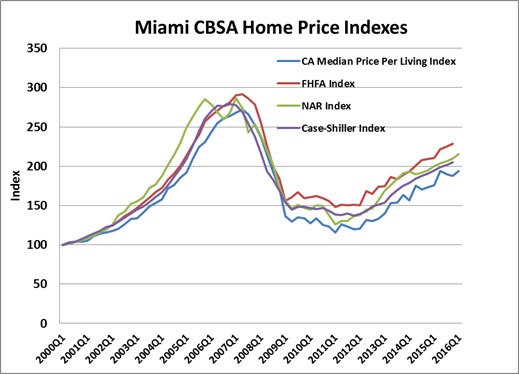
Prices are a function of time on the market and highly motivated sellers who need instant liquidity will sell for lower prices to buyers who exploit this knowledge. This leads to the question of whether such quick sales are indicative of market value? When the percentage of foreclosure driven sales is a significant proportion of the market, say 10% and above, these influences cannot be ignored.
In California, in the spring of 2008, many local markets had foreclosure numbers equal to the number of listings. Such market conditions are rare but if we are estimating current values they must be considered. The same property will typically sell for 10% or so less if sold under the label of a foreclosure.[16] In the hyper media sensitive environment of 2008 our research has shown much higher than normal discounts, perhaps as high as 25% to 50% in some markets at the trough of the housing market cycle. So, if you are in the same neighborhood where a few foreclosures occurred and are selling your home but are not a foreclosure, should the foreclosure sale be treated as a comparable property or only the non-foreclosure sales? If the foreclosure effect is considered a shorter term effect on value and the value estimate we seek is the longer term equilibrium value then it may be helpful to know the impact of foreclosures on each price index. This bias or impact on the Case Shiller index has rarely been shown, but we can estimate it in various markets using the hedonic indices that include or exclude such sales.[17] We can also estimate the constant liquidity value, that is, the value of a set of properties with expected time on the market held constant. We can also choose to estimate the index for only foreclosed properties.
In Exhibit 3 below we can observe the impact of foreclosed properties on a market like Los Angeles. From June of 2006 through June of 2008 we observe a price decline per square foot of residential housing overall of -24.7%. The REO sold property declined by 33.0% over this same period while the non REO sample declined by only 15.8%. The relative impact on any overall LA index during this time period will result in a price index approximately 50% worse than if foreclosed sales were excluded. We find a similar result in San Diego, shown in Exhibit 4.
We also find that the S&P CS Index tracks the combined index fairly well. This is shown in Exhibit 5 below. If the indexes we use influence value and hedge accounting then we are blending values together that are often unrealistic.
Should foreclosures be considered in the estimation of market value?
A property in a market dominated by foreclosures certainly competes against such sales. But a property where a few foreclosures nearby have been deeply discounted may not suffer the same price decline as buyers know whether it is a distressed sale or not. For many neighborhoods in these large cities where S&P CS indexes are utilized there are few foreclosures. For example, La Jolla and Del Mar have few foreclosures compared to southern San Diego, yet if you used an S&P CS San Diego index to estimate values for Del Mar or La Jolla, the results would be unfairly tainted by effects not appropriate for these neighborhoods.
What is the market threshold beyond which we should include foreclosure sales knowing that they are sometimes discounted by 20 % or more compared to regular values? The answer must be a function of whether those sales will set the marginal price or not. For a property owner in a hurry to sell where time on the market is a strong motivating force then foreclosed properties matter. Thus, if we defined a value for a 30 day sale in a market with 14 months of inventory, the foreclosed REO property asking prices will likely dictate price. If we are estimating market value for a normal time to sell and if the percentage of REOs on the market is a modest percentage, perhaps less than 10% of listings, then we may look to the non-REO sales as indications of value. Clearly we cannot determine the appropriate indicator of value without considering time to sell motivations.
Exhibit 3: The Impact of Foreclosed Sales on the Los Angeles Index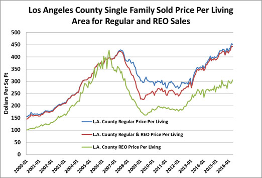
Exhibit 4: The Impact of Foreclosed Sales on the San Diego Index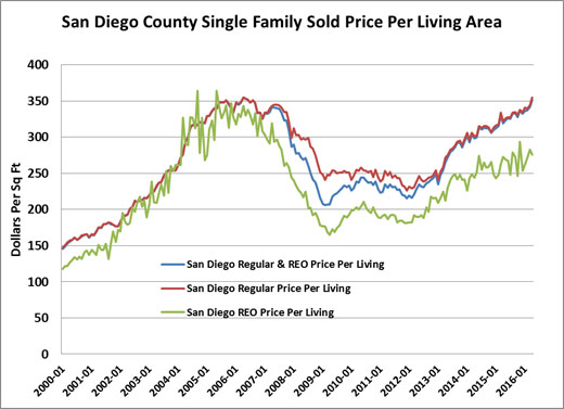
What about seasonality and prices?
Our research indicates that different markets do exhibit different degrees of variation in pricing per unit of living area over the course of a year and do so consistently. So, the time of the year when a property is sold will affect the price for which it will sell by up to plus or minus 5% from the annual average price. These monthly seasonal price factors are a direct by-product of the resulting output of how the CA models have been specified. An example of the seasonality observed for two cities, Ann Arbor and Cincinnati are shown in Exhibit 5 below. In Exhibit 6 we show how much seasonality exists in Chicago compared to San Diego. Clearly some markets, based on weather, school, tourism and employment cycles will exhibit more or less seasonality than average.
Exhibit 5: Seasonality for Two Cities

Exhibit 6: Chicago Monthly Seasonality: Price Per Square Foot of Living Area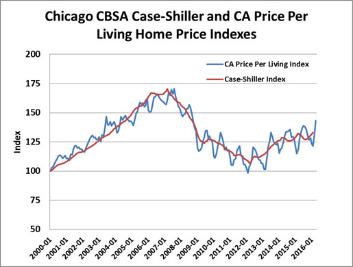
Exhibit 7: Chicago and San Diego Single Family Price Seasonality
Price indices can be developed for very granular markets. In Exhibit 8 below we show ZIP Code level indices with great variation in amplitude over the years.
Exhibit 8: ZIP Code Variations in Miami
The question of sample size is how much noise is tolerable. One way to minimize noise is to use as much sales data as is available and smooth the resulting price indexes, which enlarges temporal sample size and diminishes short term influences. For the CA Price Per Living HPIs, we use a Hodrick-Prescott Filter to smooth the inherent volatility in monthly or quarterly prices. Exhibit 9 shows the result of applying this smoothing filter to the same Miami ZIP Codes. Notice how the higher priced ZIP Codes started heading up in 2011 and 2012 while the others were going down. Real estate markets are granular and localized enough to see serious price pattern separations within the same metro market.
Exhibit 9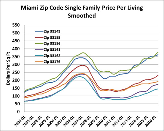
As discussed, another important benefits of using the CA Price Per Living HPI is that, by using all sales and not just those homes which had repeat sales, we can create very granular home price indexes. Exhibit 10 shows neighborhood level indexes for a single ZIP Code in Honolulu. As seen, there can be significant variation in price performance from one neighborhood to another so even ZIP Code level indexes may not provide a completely accurate picture of what the constituent homes are doing.
Exhibit 10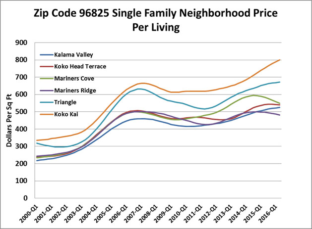
Using Information Contained in Current Listings
To bring the current market environment into the estimation of value we can enter an additional data based on current listings, as if they were sold. We know they tend to set an upper limit on value and we also know that there is a typical discount from the list prices to selling prices that allow estimates of selling prices. This adds tremendous real time information to anyone trying to predict where prices are today or where they are heading.
Such models are more robust than simple price per square foot models and yet, bring us closer to real time values. We note that if we include current listing estimated values based on known sales price to list price ratios, there will be some imbedded error but the user of such an index would know exactly how the list prices were used and how much they were discounted. This more current estimate of value moves us closer to the type of observable price we see on the stock market. It may not be the golden goose but it is as close as we can get because it utilizes all the possible information provided by all the known players.
What is our real estate worth today with normal marketing time? A hedonic model which includes current listings is one of the few ways this can be done for most of the US metropolitan markets and ZIP Codes or for any defined property type. We can also estimate what is our real estate worth with only 30 days or 60 days marketing time and provide such indices as well.
Exhibit 11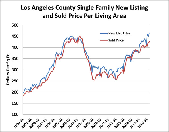
Filters and Index Types: The realities of constructing any index will require filters that screen out non-market transactions. An excellent review of filters and the methodologies provided here are discussed by Geltner and Pollakowski (2007).[18] Among the suggested filters are these:
1) Avoid flippers by eliminating very short holding period sales. For housing this could be anything under 12 months.
2) Eliminate portfolio sales with several parcels where individual transactions cannot be verified.
3) Eliminate sales where too much property information is missing, i.e. size or age.
4) Eliminate sales where the usage has changed.
5) Eliminate sales where prices are more than two deviations above normal per square foot or less than two deviations below normal. (An extreme return filter)
Types Indices which can be developed include all of the following and more: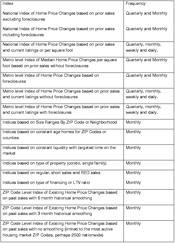
Conclusions
We can develop customized indices that allow true risk management plays, including those that represent a specific portfolio. This would include metro-wide indices or very focused submarkets and property types. Such indices would serve mortgage lenders, homebuyers, property insurance firms, investors in mortgage backed securities, municipalities whose tax revenues are tied to property values, corporate relocation companies, and a multitude of other parties who have a direct or indirect interest in the direction of residential real estate prices.
NAR’s Median Price works well enough for long term housing trends but suffers from changes in composition over time. Certainly the lower priced markets were over represented in 2007 and 2008. FHFA’s Home Price Indexes are fine for those markets with modest prices albeit with a reporting lag. S&P Case Shiller has made good progress on including a broader range of property locations but will likely suffer excessive noise in smaller or thinly traded markets and tosses out too much data to work in much more refined sub-markets. S&P Case Shiller also suffers from the bias imposed by the usual foreclosure discounts applied by buyers of REO property. Simple price indices and hedonic models provide a number of advantages over the others in that they make direct use of all available sales data, can be run for large or small geographical areas, different property types and/or different specific home characteristics, and are highly transparent with respect to methodology. In addition, by allowing significantly more sales information to be included, they lead to similar price indexes as found in thickly traded assets. Models with current listing information incorporated are one of the few ways that we really can provide daily real estate value indices and do so for nearly any reasonably sized geographic area or property type.
References for the Development of Hedonic Models
ABRAHAM, J.M and W.S. SCHAUMAN. (1991) “New Evidence on Home Prices from Freddie Mac Repeat Sales.” AREUEA Journal. 19(3), pp. 333-52.
ANAS, ALEX and S.J. EUM (1984), “Hedonic Analysis of a Housing Market in Disequilibrium”, Journal of Urban Economics, 15.
BAILEY, MARTIN, RICHARD MUTH and HUGH NOURSE (1963), “A Regression Method for Real Estate Price Index”, Journal of the American Statistical Association, 58(304), pp. 933-942.
BOURASSA, STEVEN C., FOORT HAMELINK, MARTIN HOESLI, and BRYAN D MACGREGOR (1999), “Defining Housing Submarkets”, Journal of Housing Economics, 8, pp. 160-184.
BOURASSA, STEVEN C., MARTIN HOESLI, DONATO SCOGNAMIGLIO, and PHILIPPE SORMANI (2008), “Constant-Quality House Price Indexes for Switzerland”, Swiss Finance Institute Research Paper Series, 8(10).
BOURASSA, STEVEN C., MARTIN HOESLI and JIAN SUN (2004), “A Simple Alternative House Price Index Method”, International Center for Financial Asset Management and Engineering, Geneva.
BOURASSA, STEVEN C., MARTIN HOESLI and JIAN SUN (2006), “A Simple Alternative House Price Index Method”, Journal of Housing Economics, 15(1), pp.80-97.
BOVER, OLYMPIA, and PILAR VELILLA (2002), “Hedonic House Prices Without Characteristics: The Case of New Multiunit Housing”, European Central Bank, Frankfurt.
BUTLER, RICHARD V. (1982), “The Specification of Hedonic Indexes for Urban Housing”, Land Economics, 58(1), pp. 96-108.
CASE, BRADFORD, HENRY POLLAKOWSKI, and SUSAN WACHTER (1991), “On choosing among house price index methodologies”, AREUEA Journal, 19(3), pp. 286-307.
CASE, BRADFORD, HENRY POLLAKOWSKI, and SUSAN WACHTER (1997), “Frequency of Transaction and House Price Modeling”, The Journal of Real Estate Finance and Economics, 14(1-2), pp. 173-187.
CASE, BRADFORD and JOHN QUIGLEY (1991), “The dynamics of real estate prices”, Review of Economics and Statistics, 73(1), pp. 50-58.
CASE, KARL AND ROBERT SHILLER (1987), “Prices of single-family homes since 1970: new indexes for four cities”, New England Economic Review, pp. 45-56.
CLAPP, JOHN and CARMELO GIACCOTTO (1999), “Revisions in repeat sales price indices: here today, gone tomorrow?”, Real Estate Economics, 27(1), pp. 79-104.
CLAPP, JOHN, CARMELO GIACCOTTO and DOGAN TIRTIROGLU (1991), “Housing price indices based on all transactions compared to repeat subsamples”, AREUEA Journal, 19(3), pp. 270-285.
COLWELL, PETER F. and GENE DILMORE (1999), “Who Was First? An Examination of an Early Hedonic Study”, Land Economics, 75(4), November, pp. 620-626.
DUBIN, ROBIN A. (1998), “Predicting House Prices Using Multiple Listings Data”, Journal of Real Estate Finance and Economics, 17(1), July, pp. 35-59.
FOLLAIN, JAMES R. and STEPHEN MALPEZZI (1981), “Are Occupants Accurate Appraisers?”, Review of Public Data Use, 9(1), April, pp. 47-55.
GATZLAFF, DEAN AND DAVID HAURIN (1997), “Sample selection bias and repeat-sales index estimates”, Journal of Real Estate Finance and Economics, 14, pp. 33-50.
GATZLAFF, DEAN AND DAVID LING (1994), “Measuring Changes in Local House Prices: An empirical Investigation of Alternative Methodologies”, Journal of Urban Economics, 35(2), pp. 221-244.
GOETZMANN, WILLIAM and LIANG PENG (2002), “The bias of RSR estimator and the accuracy of some alternatives”, Real Estate Economics, 30(1), pp. 13-39.
GOODMAN, ALLEN C. (1978), “Hedonic Prices, Price Indices, and Housing Markets”, Journal of Urban Economics, 5(4), pp. 471-484.
GOODMAN, ALLEN C. (1998), “Andrew Court and the Invention of Hedonic Price Analysis”, Journal of Urban Economics, 44(2), September, pp. 291-298.
GOODMAN, ALLEN C. and THOMAS G. THIBODEAU (1995), “Age-Related Heteroskedasticity in Hedonic House Price Equations”, Journal of Housing Research, 6(1), pp. 25-42.
HANSEN, JAMES (2006), “Australian House Prices: A Comparison of Hedonic and Repeat-sales Measures”, Reserve Bank of Australia, Sydney.
HOESLI, MARTIN, CARMELO GIACCOTTO and PHILIPPE FAVARGER (1997), “Three New Real Estate Price Indices for Geneva Switzerland”, Journal of Real Estate Finance and Economics, 15(1), July, pp. 93-109.
JUD, G. DONALD and DAVID WINKLER, “Return and Risk in Real Estate Futures Markets”, April, 2008, ARES Presentation Working Paper, University of North Carolina at Greensboro.
JUD, G. DONALD and J.M. WATTS (1994), “Sample Selection Bias in Estimating Housing Sales Prices”, Journal of Real Estate Research, 9(3), Summer, pp. 289-298.
KAIN, JOHN F. and JOHN M. QUIGLEY (1970), “Measuring the Value of Housing Quality”, Journal of the American Statistical Association, 65, June, pp. 532-548.
KAIN, JOHN F. and JOHN M. QUIGLEY (1972), “Note on Owners’ Estimates of Housing Value”, Journal of the American Statistical Association, 67, December, pp. 803-806.
LIM, SELWYN, MENELAOS PAVLOU (2007), “An improved national house price index using Land Registry data”, RICS Research Series, 7(11) September, pp. 212-227.
MALPEZZI, STEPHEN (2002), “Hedonic Pricing Models: A Selective and Applied Review”, Housing Economics: Essays in Honor of Duncan Maclennan, pp. 2-30.
MALPEZZI, STEPHEN, LARRY OZANNE and THOMAS THIBODEAU (1987), “Microeconomic Estimates of Housing Depreciation”, Land Economics, 63(4), November, pp. 373-385.
MILLER, NORMAN G. (1982), Residential Property Hedonic Pricing Models: A Review, Research in Real Estate, (2), pp.31-56.
MILLS, EDWIN S. and RONALD SIMENAUER (1996), “New Hedonic Estimates of Regional Constant Quality Housing Prices”, Journal of Urban Economics, 39(2), March, pp. 209-215.
NOURSE, HUGH O. (1963), “The Effect of Public Housing on Property Values in St. Louis”, Land Economics, 39, pp. 434-441.
PACE, R. KELLY and OTIS W. GILLEY (1990), “Estimation Employing A Priori Information within Mass Appraisal and Hedonic Pricing Models”, Journal of Real Estate Finance and Economics, 3, pp. 55-72.
ROSEN, SHERWIN (1974), “Hedonic Price and Implicit Markets: Product Differentiation in Pure Competition”, Journal of Political Economy, 82(1), January/February, pp. 34-55.
SHILLING, JAMES D., C.F. SIRMANS and JONOTHAN F. DOMBROW (1991), “Measuring Deprecation in Single Family Rental and Owner-Occupied Housing”, Journal of Housing Economics, 1(4), December, pp. 368-383.
WOOD, ROBERT (2007), “A comparison of UK residential price indices”, RICS Research Series, July, pp. 212-227.
Appendix 1: S&P CS Housing Market Futures and Early Adopter Returns
The Chicago Mercantile Exchange (CME) futures contracts are currently based on the S&P/Case-Shiller house price index. Contracts are available for the larger cities including but not limited to Boston, Chicago, Denver, Las Vegas, Los Angeles, Miami, New York, San Diego, San Francisco and Washington DC. The value of the futures contract is set at 250 times the S&P CS Index. At maturity the contract’s value is 250 times the average value of the index over the 3 month period ending 2 months prior to the contract month. This implies that the final settlement for August of 2008 is the average index for April through June of 2008. So we have smoothing built into the settlement and a lag so that all data adjustments can be completed. The position limits are currently 5,000 contracts.
Theory suggests that the future price will be the present value of the index, discounted at something close to the risk free rate.[19] So by presuming a risk free rate we can estimate the future values and expectations of the market. Hedgers will lay off price risk while speculators will buy or sell because they believe they can forecast price trends well enough to profit from taking a position. Futures contracts are a way for those desirous of risk shifting to transfer risks to those who wish to bear the risk.
The greater the uncertainty of the current market the more hedgers will allow speculators to profit just so they can avoid significant price risk. Risk premiums provide evidence of this uncertainty. Jud and Winkler (2008) do a nice job of examining the implications of S&P/CS trades from May of 2006 through May of 2007 on the CME. The average return was 8.57% with a standard deviation of 12.64%. Higher returns were observed in New York, Chicago and Miami and lower returns in LA and Denver.
The formula for the annualized return, AR, on futures contracts is:
ARi,t = [[(Pm/Pp)-1]+[(1+r)t-1]]*(360/t)
Pm = contract price at maturity
Pp = initial purchase price of contract
r = measure of risk free returns, usually the treasury bill rate
t = duration of the contract in days
Based on the above we can estimate percentage returns based on the change in Pm relative to Pp as follows:
Ln(Pm/Pp) where Pm and Pp are based on the price at the maturity compared to the price at the time of initial purchase.
For the period studied Jud and Winkler find the following results as shown in Exhibit A-1.
Exhibit A-1: Returns and Risks on Housing Futures Contracts based on S&P/CS 5/2006-3/2007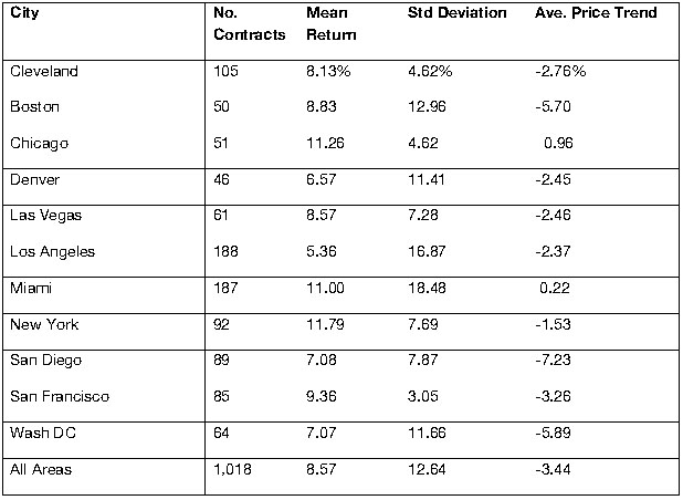

[1] See Real Estate Securities Journal, Vol. 9, November 1, Fall, 1988. A prior paper by Miller and Sklarz established the predictability of residential real estate using MLS data. See “Leading Indicators of Housing Market Price Trends,” The Journal of Real Estate Research, Fall, 1986.
[2] See “We Need a Fourth Asset Class: HEITs” D. Geltner, N. Miller and J. Snavely, Real Estate Finance, Vol. 12, No. 2, Summer, 1995
[3] Some people refer to this statistical impact as a case of the tail wagging the dog, when a small market can impact a broader index.
[4] A chart in the appendix shows that this drift is significant by region and we observe even more variation by local metro.
[5] See “A Guide to Aggregate Home Price Measures” by Jordan Rappaport, Federal Reserve Bank of Kansas City, Economic Review, Second Quarter, 2007.
[6] See www.FHFA.gov and go to the ZIP5 map.
[7] Stated another way, with large samples the noise represents residual error which cancels out so that the mean residual error or bias is zero. With small samples the noise creates distortion and bias.
[8] See Case, Pollakowski and Wachter, 1997.
[9] See “The Efficiency of the Market for Single-Family Homes” by Karl E. Case and Robert J. Shiller The American Economic Review, Vol. 79, No. 1 (Mar., 1989), pp. 125-137 and “Arithemetic Repeat Sales Price Estimators” Journal of Housing Economics, 1, 110-126, 1991 by Robert J. Shiller.
[10] See “Distressed Home Prices: The True Story,” Mortgage Banking, March 2009
[11] See “Housing Price Indices Based on All Transactions Compared to Repeat Subsamples” with C. Giaccotto and D. Tirtiroglu, AREUEA Journal, 19(3), Fall 1991, 270-285 or “Revisions in Repeat Sales Price Indices: Here Today, Gone Tomorrow,” with Carmelo Giaccotto, Real Estate Economics, 1998, 27 (1) 79-104.
[12] See Abraham and Shauman, 1993. The bias estimate is ½ to 1% per year.
[13] The Hodrick-Prescott filter is a model-free based approach to decomposing a time series into its trend and cyclical components. The H-P filter is an algorithm that “smooths” the original time series yt to estimate its trend component, τt. The cyclical component is, as usual, the difference between the original series and its trend, i.e.,
yt = τt + ct
where τt is constructed to minimize:
The first term is the sum of the squared deviations of yt from the trend and the second term, which is the sum of squared second differences in the trend, is a penalty for changes in the trend’s growth rate. The larger the value of the positive parameter λ, the greater the penalty and the smoother the resulting trend will be.
If, e.g., λ = 0, then τt = yt , t = 1,…,t.
If λ→∞, then τt is the linear trend obtained by fitting yt to a linear trend model by OLS.
Hodrick and Prescott suggest that λ = 1600 is a reasonable choice for quarterly data and that suggestion is usually followed in applied work. Monthly data? Annual data? (The greater the frequency of the data the larger the value of λ; for monthly data a value in the range of 100,000-150,000 has been suggested; for annual data a value in the range of 5-15 has been suggested.)
[14] Usually the local Board of REALTORs controls the MLS within local markets. Index construction occurs quarterly.
[15] See the working paper by Collateral Analytics titled: Why Housing Price Indices Are Super Tools Waiting to be More Fully Utilized: and How to Produce Them? Spring of 2016.
[16] See, Anthony N. Pennington-Cross, “The Value of Foreclosed Property”, Journal of Real Estate Research, Vol. 28, No. 2, 2006. Part of the discount from regular sales is the lack of a seller warranty. Part of the discount is from deterioration and property abuse and part is from the need to sell quickly.
[17] See for example, V. Been, (May 21, 2008) “External Effects of Concentrated Mortgage Foreclosures: Evidence from New York City.” Testimony before the Subcommittee on Domestic Policy, Committee on Oversight and Government Reform, U.S. House of Representatives. Center for Responsible Lending. (January 18, 2008). CRL Issue Paper: Subprime Spillover. D. Immergluck, and G. Smith. (2006) “The External Costs of Foreclosure: The Impact of Single-Family Mortgage Foreclosures on Property Values,” Housing Policy Debate 17 (1): 57-79. Lin, Z, E. Rosenblatt, and V. Yao. (2009) “Spillover Effects of Foreclosures on Neighborhood Property Values,” Journal of Real Estate Finance Economics 38 (4).
[18] See “A Set of Indexes for Trading Commercial Real Estate Based on the Real Capital Analytics Transaction Prices Database” by David Geltner and Henry Pollakowski, MIT Center for Real Estate, Commercial Real Estate Data Laboratory, Release 2, September 26, 2007.
[19] See Fama, E. and K. French, “Commodity Futures Prices: Some Evidence on Forecast Power, Premiums and the Theory of Storage”, Journal of Business, 1987, 60:1, 55-73. John Maynard Keyes (1930) in a “Treatise on Money” provided the original theoretical basis for pricing futures.
Download a PDF file of this research paper here.