by Michael Sklarz, Ph.D. and Norm Miller Ph.D.
Abstract
There are a variety of house price indices that are useful for the market. While large scale metro indices are most often discussed by the media, consumers along with the industries affected by home price trends could and should use these to develop new financial products including home price insurance, price risk hedging, credit score modeling and mortgage default risk modeling. The mortgage and insurance industries should use a large array of new tools to greatly improve the informational efficiency of risk modeling and our understanding of home price trends at the very micro level and for a variety of specific concerns and amenities. Here we provide a set of examples of what is possible in this arena.
Introduction
Bailey, Muth and Nourse, in 1963, published the first methodology paper suggesting that we could track housing price trends through use of a repeat sales index. Later, Case and Shiller (1988) capitalized on this methodology with their production of various major housing market indices, now widely known and reported. In a Google Scholar search of housing price index related research there are 8030 academic papers with 2910 focused on methodologies from hedonic regression methods to every conceivable variation that econometric experts can dream up.[1] Yet, housing price indices, HPIs, remain an underutilized tool in the market place and the media tends to focus on the large general indices, which are not really applicable to the majority of business or consumer decisions.[2] Here we provide some illustrations on HPIs from the aggregate to micro levels and for various types of properties and categories. We also briefly review the methodologies available and some future HPI possibilities.
The Usefulness and Relevancy of HPIs Increases as Disaggregation Increases
HPIs could be utilized to produce an array of useful financial products from home price insurance, to mortgage default insurance to individual credit models and other hedging tools. It has been well established that home price declines significantly increase mortgage default, which suggests that price risk insurance could help mitigate mortgage insurance risks if appropriate indices can be developed.[3] For example, if one could buy a put option on their own geographic and property type market they may be able to hedge against price declines. For the less sophisticated consumer, an insurance company might simply sell property price insurance and do the hedging for a fee. Mortgage insurance companies, knowing that strategic defaults ramp up when prices decline significantly might use tradeable HPIs to hedge against this portion of the mortgage insurance risk. Local HPIs might also be used to adjust and estimate home equity to predict negative equity or to predict positive equity which could feed into a credit score and probability of default model. Everyone’s credit score could reflect not just payment history and income but the chance of negative equity in their home as well.
In 1988 Miller, Sklarz and Stedman proposed the development of options that could be traded to help hedge against home price volatility. Yet, the data was not that available nor as robust as it is today, so the idea languished. Later in 1993 Case, Shiller and Weiss presented the same idea and later tried to help develop an options market on the Chicago exchange based on twenty metro level housing indices. One impediment to the implementation of such an idea is that all housing markets are very local. For example, in a 2009 article for the Mortgage Bankers Association, Miller and Sklarz compared Zip Code level price changes to those reported at the Metro level by Case and Shiller. From that article we produced a chart just like Figure 1 below, updated, that shows that two thirds of the Zip Codes had declined less than suggested by Case-Shiller while one third had declined more. This is for the recent Q1, 2010 through Q1, 2016 recovery phase of the market and we see similar results for most time periods and most markets.
Figure 1: Zip Code Price Changes Compared to the Case Shiller Metro Result for San Diego 2010 Q1 through 2016 Q1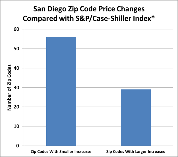
Then in Figure 2 below we provide a similar comparison to the metro level index for San Diego for the prior “market crash” period. Here even over several years we observe a small percentage of Zip Codes with a significant price change can sway an entire metro index. In this chart we see a large bar representing the Case Shiller Index for that time period at around -37%. 59% of the Zip Codes declined less than this and a few much less than this.
Figure 2: Metro Versus Zip Code Price Change over 7 years in San Diego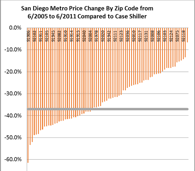
The obvious conclusion is that metro level price trends do not affect all houses the same and also that a hedging instrument assumed to apply to a given homeowner might actually have experienced the opposite market trend, if a more localized HPI were possible. Metro and CBSA indices are not that useful for individuals, investors or lenders.
To illustrate this point, look at Figure 3 below where we compare six levels of geographic HPIs from the State of California, down to the CBSA, County, City, Zip and then even smaller, a neighborhood. Zip Code level analysis was recently suggested by researchers at the Federal Housing Finance Agency, but even neighborhood level analysis or individual home analysis is possible today.[4] Collateral Analytics has defined over 400,000 neighborhoods in the US by mining data from local multiple listing services along with several other parameters.[5] What becomes clear is that the state and CBSA were experiencing negative price trends while homes in the neighborhood shown were experiencing positive price trends. The more localized the market, the more applicable an index is to any particularly located home. Here we simply show indexed median single family home sold prices for the HPIs.
Figure 3: Geographic Based HPIs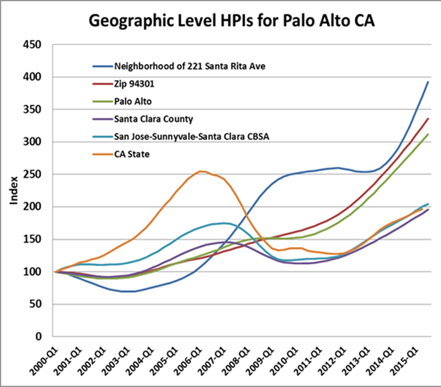
In fact, we can dig even deeper and generate not only a neighborhood price index but also one based on retrospective Automated Valuation Models (AVM)[6] values to generate a value index, low and high index for a particular home as we see in Figure 4 below. The AVM used here is the Collateral Analytics CA Value AVM of a given subject property. There is some noise[7] in these estimates but a smoothing[8] function can be applied to eliminate much of the noise. Such an index can be used to estimate quite accurately the level of positive equity as a percentage of the home value, given mortgage document integration with the HPI model.[9]
Figure 4: Geographic Based HPI at the Lowest Micro Level: An Individual Home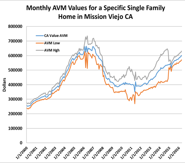
Methodology Alternatives
There are several common methods to generating a house price index. All require filters to scrub out extreme values that might be a result of data mistakes or non-market transactions. For example, a sale for $1 from Appleby to another Appleby would be filtered out because it is an extreme value for a 2500 square foot home and also because the last name is the same. Other extreme values are typically filtered as they could be an error or non-representative. The typical approach is the use two standard deviations from the mean for a set of key variables including but not limited to living area size and age, and lot size. By using two standard deviations we exclude the 5% most extreme values and retain 95% of the possible sample. With respect to the calculation of the index itself, there are several common methods including:
-Median Home Price: This is simply the middle price of a distribution and if it is similar to the mean or average then the distribution is fairly symmetric above and below the mean and possibly normal. The problem with using a median, or mean is that it does not control for differences in the size of quality of the home over repeated samples. Thus, it is a very crude measure as an index.
-Mode Home Price: This is simply the most frequent price and if it matches the median then it is fairly representative of the typical home in a given area.
-Mean Home Price: This is a common index produced by trade associations without controls for variations in size or quality. It is useful in judging affordability relative to income and current interest rates.
-Mean Home Price Per Square Foot of Living Area: By adjusting for size this index provides a better control over the mix of observations and is thus a better indication of true price trends for the typical owner in a particular market. For small geographic areas this index will produce a price trend very much in line with more sophisticated techniques.
-Constant Quality Home Price: Using a hedonic pricing regression model this index attempts to control for the most common elements driving value including size, age, baths, bedrooms, lot size and other features. Once a hedonic model is established with a good fit and high explanatory value then it can be used to judge the change in prices for a more constant bundle of attributes. Because of such controls it can be used on a small market area or larger geographic areas.
-Constant Liquidity Home Price: Home prices can vary simply because some sellers need a quicker sale while others have less urgency and so the list price relative to true market value can affect the time on the market. By controlling for the time on the market we can develop a constant liquidity home price index. This can be done by filtering out extremes or by focusing on a certain time period within which sales take place. There are many variations on how to do this, but the idea is the control the time on the market and use a selected matching set of sales as representative of the current market prices. One simple variation on this would be to separate regular sales from distress sales.
-Repeat Sales Index: This is a method that uses overlapping samples of identical properties that have sold at least twice with filters for very short time periods. Repeat sales are thought to represent typical property owners in a given geographic area, however, they may be biased if they do not control the level of distress in the mix or the effects of unusual mixes of units selling at one particular point in time, such as price tiers or size mixes. The well-publicized Case Shiller index is a repeat sales index.
While constant quality hedonic regression based models techniques work well, they require much larger geographic areas for sophisticated development. It turns out that price per square foot of living indices produce nearly identical results for homogeneous submarkets or well defined neighborhoods. The reason is quite straight forward. Most of the variation in average prices over shorter to intermediate time periods is correlated with home size. Below we generate some HPIs using price per square foot and here we break the HPIs into property types, single family detached, condominium and multifamily properties. Note that the general movement is the same but there are variations in the magnitudes and spreads over time. Again, the point is to use an HPI for as localized a market as possible but also not to presume that all residential category property types are perfectly in sync. In late 2007 single family prices in Miami had started falling while easy subprime lending targeted at condos continued to drive up these prices until a bubble popped and condo’s plummeted faster and further than any other residential type during 2008.
Figure 5: Property Type HPIs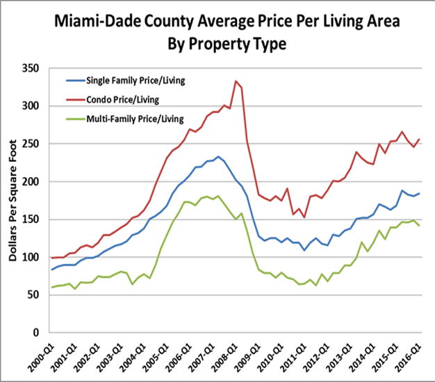
Just as price per square foot may produce a reliable HPI other physical indices can also be based on bedrooms. See Figure 6 below. Such an index might be very appropriate for a student rental market where units are rented by the bedroom. Such an index also provides information on relative demand by size tier.
Figure 6: Physical Size Tier by Number of Bedrooms HPI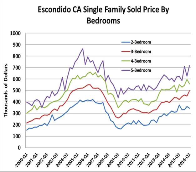
Further examples of HPIs which can be generated include those for specific amenities such as floor level on a condo, whether the home has a mother-in-law suite, mountain-view, water view or water front property. Such indices can also be used to estimate the impact of negative externalities from natural or man-made causes such as oil spills or airports. In Figure 7 we generate simply the impact of being on water as opposed to off water in the same general neighborhood. Here the premium is shown to be 25% to 40%, depending on the temperature of the current market conditions.[10]
Figure 7: Specific Property Amenity HPIs: The Example of Waterfront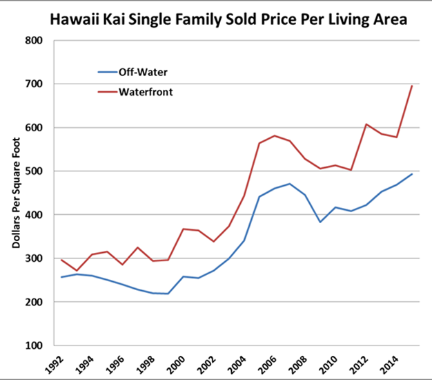
One of the most important differentiators of home prices is the type of sale. Not only do these contaminate indices that are supposed to be indicative of regular non-distressed sale price trends, but there are systematic reasons why such differences persist. REO sales are from lenders that have foreclosed and not only are they typically priced for quick (under 60 day) sales but they are generally sold as-is. This lack of a warranty requires a discounted price which is typically 15% to 22% but can range as high as 50% or more in distressed markets and as low as 5% to 10% in recovering markets with distress investors fighting over dwindling inventories. Short sales are merely sales with approval to be sold below mortgage balances and these are also typically sold at a discount. The way one would use such indices is by using the one most likely to match the selling circumstances of the property being analyzed.
Figure 8: Type of Sale HPI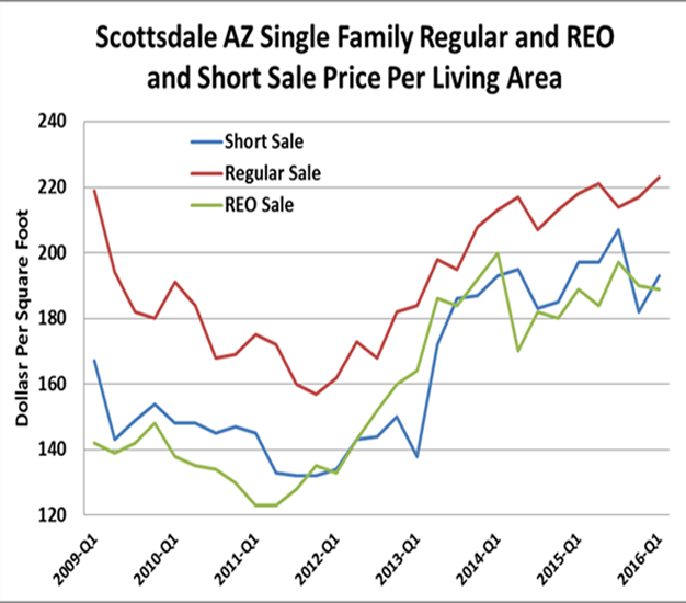
We can also produce HPIs by vintage. Generally, as we see below in Figure 9, newer property is worth more per square foot and contains qualitatively better home features, or it is correlated with property condition as we see in Figure 10, discussed next. Vintage captures significant variation in price. One could easily use such an index based on properties from the same area to estimate current values, changes in values or the impact of newer stock on the older stock.
Figure 9: Property Price Per Living Area By Year Built HPIs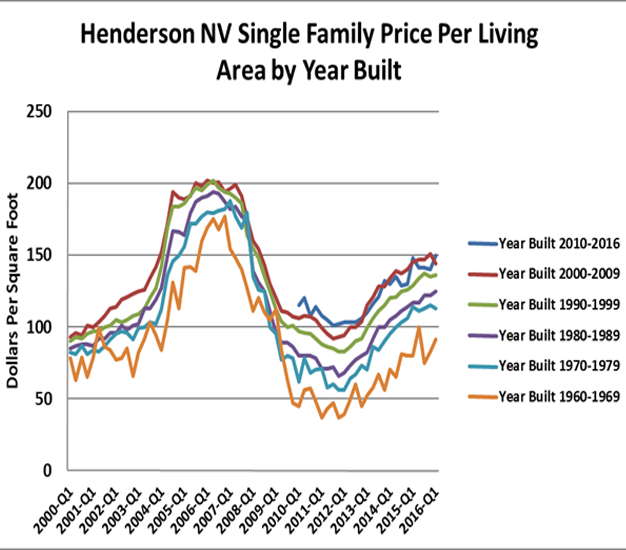
Last, we can produce HPIs for specific qualitative differences in properties. For example, by mining descriptors from listing agent data or prior appraisals we can estimate differences in property condition and how much this affects selling price. This is shown in Figure 10 below following the standard appraisal condition rankings. Note how the spread from poor to good condition narrowed during the easy underwriting high leverage period of 2000 through 2005, but as real equity entered the picture and underwriting became more constrained, spreads subsequently widened. Such HPIs help us predict spreads based on combining qualitative information with market conditions.
Figure 10: Property Condition HPIs 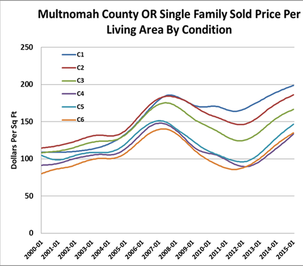
Conclusions
Housing Price Indices could be produced and disseminated the same way we do stock prices with all the market data that helps us understand the direction of the market, such as volume of trading, bid ask spreads, volatility indices and so forth. These indices are continuously being improved, and produced with very little time lag, but still they remain under-utilized as tools for valuation, predicting price trends, estimating equity and credit scores and risks of default on an on-going basis. Such an important asset as housing deserves a little more transparency in order to help markets work more efficiently.
If we took a sample of properties and applied all the relevant indices above, we could do an excellent job of estimating values or tracking the likely path of price trends for each property type. One might argue that all property is unique, but that is not really the case. Most property has more than enough peers and substitutes that we can dissect any neighborhood or Zip Code and city and explain which traits are moving prices more than others or how much each matters. Whether the price trends by vintage or price tier or size are in sync is the subject of another working paper from Collateral Analytics to be available soon.
References
Agarwal, S., I. Ben-David, V. Yao (2015) “Collateral Valuation and Borrower Financial Constraints: Evidence from the Residential Real Estate Marke” Management Science 61(9):2220-2240. http://dx.doi.org/10.1287/mnsc.2014.2002
Bogin, Alexander N, William M. Doerner and William D. Larson, “Local House Price Dynamics: New Indices and Stylized Facts” FHFA working paper, March 18, 2016
Bailey, M, R. Muth and H. Nourse, (1993) “A Regression Method for Real Estate Price Index Construction” Journal of the American Statistical Association, 58, 922-942.
Case, K.E. and R. J. Shiller, “The Efficiency of the Market for Single-Family Homes” NBER Working Paper No. 2506 (Also Reprint No. r1229), Issued in February 1988 NBER Program(s): later published in the American Economic Review (1989)
Case, K., R. Shiller and A. Weiss “Index-Based Futures and Options Markets in Real Estate” The Journal of Portfolio Management, 1993, 19:2, 83-92
Miller, N., M. Sklarz, and B. Stedman, “It’s Time for Some Options in Real Estate”, Real Estate Securities Journal, 9, 1 (1988), 42-51.
Miller, N. and M. Sklarz “Distressed Home Prices: The True Story” Mortgage Bankers Magazine, March, 2009.
Thibodeau, T. Journal of Real Estate Finance and Economics, 1997 “Housing price indices” Special Edition with 13 articles.
Wang, F.T., and P. M. Zorn “Estimating House Price Growth with Repeat Sales Data: What’s the Aim of the Game?” Journal of Housing Economics, 6:2, June 1997, 93-118.
*Forthcoming in Real Estate Issues, 2016.
[1] Tom Thibodeau was the Editor of a special issue of the Journal of Real Estate Finance and Economics in 1997 focused entirely on housing price indices.
[2] William Wheaton of MIT said in a 1998 lecture that “no one owns the typical home in America so why do we care about an average that applies to almost no one.”
[3] See Agarwal, Ben-David, Yao (2015)
[4] See Bogin, Dorener and Larson (2016) in references.
[5] For example, school districts, postal carrier routes and physical boundaries, similar home vintages and prices ranges. There are typically 10 to 15 neighborhoods in a Zip Code.
[6] AVM – Automated Valuation Model (AVM) is the name given to a service or tool that can provide real estate property valuations using mathematical modelling combined with a database of real estate transactions and property and location attributes. Most AVMs calculate a property’s value at a specific point in time by analyzing values of comparable properties using one of several methods that include hedonic methods, appraisal emulation and others.
[7] Noise – Unexplained variation or randomness which is found within a data series.
[8] Smoothing – Statistical technique used to remove short term irregularities in a time-series to help improve the accuracy and identify the underlying trend.
[9] It is not hard to estimate mortgage balances, but one must be careful to research second mortgage balances as well and equity lines of credit that have been drawn down or might be utilized.
[10] At Collateral Analytics we define market conditions from distressed to hot, and these are highly correlated with time to market and general price trends. During stronger markets it appears that water front properties become relatively more desirable with larger premiums.